A Practical Guide to VLOOKUP with Multiple Criteria in Excel

VLOOKUP() is one of Excel's most widely-used functions. It allows you to look up and retrieve data from a specific column in a table. It's a fundamental tool for merging data from different sheets or finding related information.

But VLOOKUP() has a well-known limitation: it can only search based on a single condition. This becomes a problem when you need to match multiple conditions to find the right data—a common scenario in any serious spreadsheet work.

In this article, we’ll see how you can overcome this limitation. We'll cover the classic formula-based techniques, and then introduce a modern, AI-powered approach that gets the job done in seconds, without any formulas. If you are new to Excel, mastering these concepts is crucial for efficient data management.

VLOOKUP() Basics

Before we tackle multiple criteria, let's quickly review the basic VLOOKUP() syntax:

=VLOOKUP(lookup_value, table_array, col_index_num, [range_lookup])

In the above formula:

• lookup_value is the value you want to search for.
• table_array is the range of cells that contains the data. The lookup value must be in the first column of this range.
• col_index_num is the column number in the range from which you want to retrieve the value.
• range_lookup is a logical value (TRUE for an approximate match, FALSE for an exact match). You'll almost always use FALSE.

Let's see it in action. We have a sheet of employee data and want to find an employee's first name using their ID number.

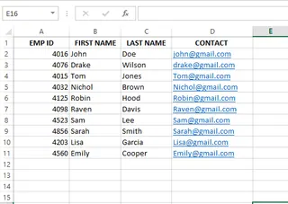
We enter the ID 4032 in cell F6. In cell G6, we use the following formula:

=VLOOKUP(F6, A2:D11, 2, FALSE)

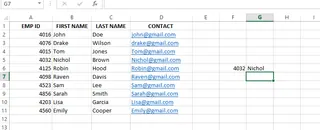
Excel finds 4032 in the first column of our table, moves to the 2nd column, and returns the name "David". Simple and effective. But what if we needed to find a value using two or more criteria?

How to Handle Multiple Criteria: The AI vs. The Manual Way

When faced with multi-criteria lookups, you have two paths: the modern, AI-powered way, or the traditional, formula-based way. Let's start with the simplest and fastest solution.

The Modern Way: Multi-Criteria Lookups with an AI Assistant

Instead of building complex formulas, you can use an AI Excel Agent like Excelmatic to do the work for you. The process is incredibly simple: upload your spreadsheet and ask your question in plain language.

Let's take a common business problem: finding a specific sales amount based on the customer, product, and date.

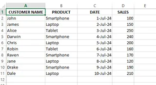
Instead of writing a formula, you would simply upload this file to Excelmatic and ask:

"What is the sales amount for James for a Laptop on 02-Jul-24?"

Excelmatic understands your request, scans the data, and gives you the answer instantly.

Here’s the comparison:

• Traditional Method: Requires creating a new "helper" column, concatenating data from three different columns, carefully writing a VLOOKUP formula that matches the new concatenated format, and handling potential data type issues (like dates turning into numbers).
• Excelmatic Method: Ask one question.

The AI approach eliminates the need for intermediate steps, complex syntax, and troubleshooting. It's faster, less prone to error, and lets you focus on the question you want to answer, not the formula you need to build.

The Manual Method: Using Formulas for Multi-Criteria Lookups

If you prefer to build the solution yourself or want to understand the mechanics behind it, here are the classic formula-based techniques.

Method 1: VLOOKUP() with a Helper Column

This is the most common manual approach. You create a "helper" column that combines your multiple criteria into a single, unique value. Then, you perform a standard VLOOKUP() on that column.

Using our sales data example, we want to find the sales amount based on Customer Name, Product, and Date.

Step 1: Create the Helper Column

Insert a new column (e.g., in column A) and combine the criteria. We'll join the values from Customer Name, Product, and Date using the & operator. It's good practice to use a separator like | to prevent incorrect matches (e.g., "AB" & "C" is the same as "A" & "BC").

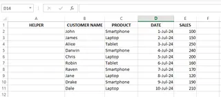
The formula in the new column A would be:

=C2&"|"&D2&"|"&E2

When you concatenate a date, Excel often converts it to its underlying serial number. To keep the date format readable and ensure a correct lookup, it's better to use the TEXT() function.

The improved formula is:

=C2&"|"&D2&"|"&TEXT(E2, "DD-MM-YY")

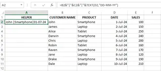
Drag this formula down to fill the entire column.

Step 2: Perform the VLOOKUP

Now, you can use a standard VLOOKUP() that references your criteria cells and looks for a match in the new helper column.

=VLOOKUP(H2&"|"&I2&"|"&TEXT(J2, "DD-MM-YY"),$A$2:$F$11, 6, 0)

This works, but it requires modifying your source data, which isn't always ideal.

Method 2: VLOOKUP() with the CHOOSE() function

A more advanced technique involves creating a "virtual" helper column using the CHOOSE function, so you don't have to alter your table. CHOOSE can build a new table array in-memory for VLOOKUP to use.

The syntax for CHOOSE is: CHOOSE(index_num, value1, [value2], ...).

Let's use this dataset of student scores:

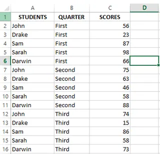
To find a student's score for a specific quarter without a helper column, we can use this array formula:

=VLOOKUP($E2&"|"&F$1, CHOOSE({1,2}, $A$2:$A$16&"|"&$B$2:$B$16, C2:C15), 2, FALSE)

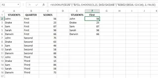
Here’s how it works:

• CHOOSE({1,2}, $A$2:$A$16&"|"&$B$2:$B$16, C2:C15) creates a virtual two-column table. The first column is a concatenation of the Student Name and Quarter, and the second column is the Score.
• The VLOOKUP then searches this virtual table.

This is powerful but also complex and can be difficult to debug.

An Alternative to VLOOKUP: INDEX() and MATCH()

For decades, the combination of INDEX() and MATCH() has been the preferred method for advanced lookups. It's more flexible than VLOOKUP() and can handle multiple criteria natively with array formulas.

• MATCH() finds the position of a value in a range.
• INDEX() returns a value from a specific position in a range.

Let's use this employee dataset to find the position of John, who is 25 and lives in Chicago.

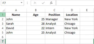
Here are our criteria:

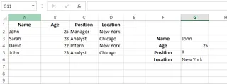
The formula in cell G5 is:

=INDEX(C2:C5,MATCH(1,(G3=A2:A5)*(G4=B2:B5)*(G6=D2:D5),0))

This is an array formula, so you might need to press Ctrl + Shift + Enter in older Excel versions.

This formula works by creating arrays of TRUE/FALSE values for each condition, multiplying them to find the row where all conditions are TRUE (which evaluates to 1), and using MATCH to find that row's position. It's extremely powerful but has a steep learning curve.

Final Thoughts

We've covered the classic techniques for multi-criteria lookups—helper columns and the powerful INDEX/MATCH combination. Mastering these formulas will certainly make you more confident in handling complex datasets.

However, the landscape of data analysis is evolving. AI tools like Excelmatic offer a paradigm shift, moving the focus from "How do I write the formula?" to "What question do I want to ask my data?". By handling the complex mechanics in the background, these tools empower you to find insights faster and more intuitively than ever before.

Ready to skip the formulas and get instant answers from your data? Try Excelmatic for free today and experience how AI-powered data analysis can transform your workflow.

Whether you stick with the formulas or embrace the AI assistant, the goal is the same: to turn your data into answers.

FAQ

Can VLOOKUP() return multiple values?

VLOOKUP() itself cannot return multiple values. For that, you would need to use other functions like FILTER (in Microsoft 365) or a combination of INDEX(), SMALL(), and ROW() in an array formula.

How do you create a two-way lookup with VLOOKUP()?

You can combine VLOOKUP() and MATCH() to create a two-way lookup, where MATCH() dynamically finds the column index number for VLOOKUP(). However, a two-way INDEX/MATCH/MATCH is generally more robust.

How do you perform a case-insensitive lookup in Excel?

By default, VLOOKUP(), MATCH(), and XLOOKUP() are all case-insensitive. For a case-sensitive lookup, you would need to use a function like EXACT() within an array formula.