A Smarter Way to VLOOKUP: The Modern Guide to Data Lookups in Excel

You’ve probably heard about VLOOKUP(). It’s one of the most well-known (if not the most well-known) functions in Excel. For decades, it has been the go-to solution for a notoriously tricky and time-consuming problem: finding a piece of information in one list and retrieving a related piece of information from another. VLOOKUP is Microsoft’s way of giving you back a lot of time.

But what if there was an even faster way? In this article, we’ll demystify how VLOOKUP() works and walk you through its most common uses. We'll also introduce a modern, AI-powered alternative that can deliver the same results without you ever having to write a formula again.

What Does VLOOKUP() Do?

Let's get clear on what VLOOKUP() actually does. In essence, it searches for a value in the first column of a table (or range of cells) and returns a value from another column in the same row.

Think of it like this ask: "Find this item in my list, and give me something else from the same row."

To do this, you need to provide four important arguments:

=VLOOKUP(lookup_value, table_array, col_index_num, [range_lookup])

• lookup_value: The value you want to search for.
• table_array: The range of cells containing your data (including both the column to search and the column(s) to return).
• col_index_num: The column number (starting from 1 for the leftmost) in the table_array from which to return the value.
• [range_lookup]: Optional. Enter FALSE for an exact match (this is usually what you want), or TRUE for an approximate match.

VLOOKUP() is a function where you have to understand the arguments. Not all functions are like this, but VLOOKUP() definitely is.

Excel VLOOKUP() Basic Example

Let’s put VLOOKUP() to work. Suppose you have a simple table of products and prices, like so:

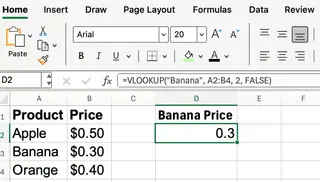
Say you want to know the price of a banana. You can use:

=VLOOKUP("Banana", A2:B4, 2, FALSE)

• "Banana" is the value you're searching for.
• A2:B4 is the data range.
• 2 tells Excel to return the value from the second column, which is Price.
• FALSE means you want an exact match.

This formula will return $0.30. Simple enough, but you had to know the exact syntax and the position of the "Price" column.

The AI Alternative: Just Ask a Question

Now, let's achieve the same result with an AI-powered tool like Excelmatic. Instead of writing a formula, you simply use plain language.

1. Upload your spreadsheet to Excelmatic.
2. Ask the question: "What is the price of a banana?"

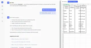
Excelmatic understands your request, finds "Banana" in your data, and instantly returns the answer: $0.30. There's no syntax to remember, no cell ranges to define, and no column numbers to count.

VLOOKUP() with Cell References

In that last example, we hard-coded the lookup value. In practice, you'll often want to reference a cell. This makes your formula dynamic. For example, if you enter "Orange" in cell D2, you can use:

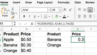
=VLOOKUP(D2, A2:B4, 2, FALSE)

Now, anytime you change the value in D2, the formula fetches the corresponding price.

With an AI tool like Excelmatic, this process is just as intuitive. You can ask, "For each item listed in column D, find its price from the product table." Excelmatic will perform the lookup for every item and generate a new table with the results, all from a single command.

VLOOKUP() Using Exact vs. Approximate Match

Now you might be wondering about that fourth argument, [range_lookup]. Most of the time, you’ll want FALSE for an exact match.

• Use FALSE for things like product IDs, names, or codes where you need a precise match.
• Use TRUE for numerical ranges (like tax brackets or grading scales) where you want the closest value without going over. Important: Your lookup column must be sorted in ascending order when using TRUE.

Let’s see an approximate match example. Suppose you have this table for tax rates:

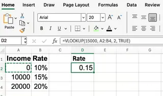
If your income is $15,000, the formula is:

=VLOOKUP(15000, A2:B4, 2, TRUE)

Excel will find the closest value less than or equal to 15000 (which is 10000) and return 15%.

Once again, the AI approach simplifies this. You would just ask, "Based on the tax table, what is the tax rate for an income of $15,000?" The AI handles the logic of finding the correct bracket without you needing to specify TRUE or worry about sorting your data first.

Common Pitfalls and How to Avoid Them

VLOOKUP() is powerful, but it has limitations that can trip you up. This is where the difference between traditional formulas and modern AI tools becomes crystal clear.

• Limitation 1: Only searches left-to-right. VLOOKUP() always searches in the first column of your table_array. If you need to look up a value and return data from a column to its left, VLOOKUP can't do it.

  • The AI Solution: AI agents like Excelmatic don't have this limitation. You can ask it to find a value in any column and return data from any other column. You refer to columns by their headers (e.g., "Price," "Product ID"), not their position.

• Limitation 2: The column number is static. If you insert or delete a column in your table, your col_index_num will be wrong, breaking your formula or, worse, returning incorrect data.

  • The AI Solution: Since you ask for data using column names ("Find the Price"), your request remains valid even if you restructure your table. The AI adapts automatically.

• Limitation 3: Handling errors is manual. If VLOOKUP() can’t find a value, it returns an ugly #N/A error. To fix this, you have to wrap your formula in another function, IFERROR().

  • The AI Solution: Excelmatic handles this gracefully. If a value isn't found, it simply reports that, or you can specify what to do in your prompt, like "...if a price isn't found, just write 'Not available'." No nested formulas needed.

Let's look at the IFERROR fix:

=IFERROR(VLOOKUP(D2, A2:B4, 2, FALSE), "Not found")

This works, but it adds another layer of complexity. The AI approach avoids this entirely.

VLOOKUP() vs. INDEX/MATCH vs. XLOOKUP()

To overcome VLOOKUP's limitations, Excel users have traditionally turned to other functions.

• INDEX() + MATCH(): This combination is more flexible. It can look up values in any direction (left, right, up, or down) and isn't broken by inserting or deleting columns. However, it requires nesting two different functions, making it more complex to write.

• XLOOKUP(): This is the modern successor to VLOOKUP. It combines the simplicity of VLOOKUP with the power of INDEX/MATCH. It can look left, has a built-in "if not found" argument, and is generally more intuitive. It's a fantastic function, but it's only available in newer versions of Excel (Excel 2021, Microsoft 365).

Traditional Functions vs. The AI Agent Approach

Think of VLOOKUP, INDEX/MATCH, and XLOOKUP as different tools in a toolbox. To be effective, you need to learn which tool to use for which job and how to use it correctly.

An AI agent like Excelmatic is like having a master data analyst at your side. You don't need to know about the tools in the toolbox. You just describe the outcome you want—"Merge these two tables based on the 'Employee ID' column," or "Create a chart showing sales by region"—and the AI selects and uses the best method to get it done instantly.

Conclusion: Work Smarter, Not Harder

VLOOKUP() is a fundamental Excel skill, and understanding how it works provides a great foundation for data manipulation. For years, mastering its intricacies, along with those of INDEX/MATCH and XLOOKUP, was a hallmark of a proficient Excel user.

However, the landscape is changing. The future of productivity lies in tools that let you focus on your goals, not the syntax required to achieve them. While learning formulas is still a valuable skill, AI-powered solutions like Excelmatic offer a more direct path from question to insight. They handle the complexity behind the scenes, allowing you to perform powerful data lookups, analysis, and reporting simply by asking.

Ready to say goodbye to complex lookup formulas? Try Excelmatic today and start finding the answers you need by simply asking for them.

So, the next time you face a complex lookup task, by all means, use VLOOKUP if you're comfortable with it. But also know that there's a smarter, faster way waiting for you—one that speaks your language.