A Guide to INDEX MATCH with Multiple Criteria in Excel

A couple of years ago, I worked on a marketing campaign analysis where I had to compare sales performance across multiple regions. The data was spread across multiple Excel sheets, and I had to pull specific product sales numbers into a single summary report. At first, I tried manually searching and copying the data, but it was not as easy as I thought. If there’s one wrong row, the whole report could fall apart.

That’s when I found INDEX MATCH. It took me a few tries to get the formula right, but it became a part of my routine once I saw how easily it could locate and pull the exact numbers I needed. For a long time, it was my go-to solution for complex lookups.

Today, while INDEX MATCH remains a powerful skill, the landscape is changing. AI-powered tools now offer a way to get the same results without writing a single formula. In this article, I’ll explain how you can master multi-criteria lookups using the traditional INDEX and MATCH functions, and also show you how a modern tool like Excelmatic can achieve the same outcome in a fraction of the time.

A Refresher on INDEX MATCH

INDEX MATCH is a shorthand way of talking about the combination of two Excel functions that work together to perform advanced lookups. We could also refer to this as INDEX(MATCH()), but I'll use INDEX MATCH in this article. Now, let's take a look at each in turn:

The INDEX() function retrieves the value of a cell based on its position within a specified range. Here’s its syntax:

=INDEX(array, row_num, [column_num])

Here:

• array is the range of cells from which you want to retrieve a value.
• row_num is the row number in the array from which to return a value.
• column_num (optional) is the column number in the array from which to return a value.

The MATCH() function identifies the relative position of a value within a range. Its syntax is:

=MATCH(lookup_value, lookup_array, [match_type])

Here:

• lookup_value is the value you want to find.
• lookup_array is the range where the function searches for the value.
• match_type is optional. 0 finds an exact match and is what we'll use most often.

How to combine INDEX() with MATCH()

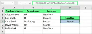
By nesting MATCH() within INDEX(), we can create a dynamic lookup. Let’s understand this with an example: Suppose you want to find the department of "David Wilson" in the dataset. Instead of hardcoding the row number in INDEX(), use MATCH() to determine it:

=INDEX(C2:C6, MATCH("David Wilson", A2:A6, 0))

In the above formula, MATCH("David Wilson", A2:A6, 0) returns 4, which is the row position. And INDEX(C2:C6, 4) retrieves the value from the 4th row of the range C2:C6, which is "Seattle".

INDEX MATCH vs. VLOOKUP()

Now that you know how INDEX() and MATCH() work, let’s see why INDEX MATCH is often a better choice than the more common VLOOKUP().

• Flexibility: Unlike VLOOKUP(), which requires the lookup column to be the first one on the left, INDEX MATCH allows you to retrieve data from any column, regardless of its position.
• Stability: Formulas using VLOOKUP() can break if columns are inserted or deleted, as they rely on a static column index number. INDEX MATCH is more robust because it references the return column directly.
• Performance: INDEX MATCH can be faster on large datasets as it processes only the lookup and return columns, whereas VLOOKUP() can select a larger array of data.
• Clarity: With INDEX MATCH, you don’t have to manually count column numbers. You specify the lookup column and the return column, which can make the formula easier to read.

INDEX MATCH with Multiple Criteria: The Traditional Way

I often have to work on datasets that contain duplicate entries, and finding values based on more than one condition is a common task. INDEX MATCH can handle these scenarios, but it requires a more advanced formula structure. Let me walk you through it step by step.

Set up data for multiple criteria

First, create your dataset and make sure it is well organized into a table with clear headers for each column. Each row should represent a unique record, and each column should contain a specific data attribute.

For example, here’s a sample dataset:

Write the formula for multiple criteria

The standard INDEX MATCH formula only works with one criterion. To handle multiple criteria, we need to adapt it into an array formula.

Here’s the basic syntax for this:

{=INDEX(return_range, MATCH(1, (criteria1=range1) * (criteria2=range2), 0))}

Here:

• return_range is the range from which the value will be returned.
• criteria1, criteria2 are the conditions to be satisfied.
• range1, range2 are the column ranges to check the criteria against.
• The * operator acts as an AND condition, creating an array of 1s and 0s. MATCH(1, ...) then finds the first row where all conditions are true (resulting in a 1).

Let's look at two methods to apply this.

Method 1: Use a helper column

If you're not comfortable with array formulas, a helper column can simplify the process. It works by combining multiple criteria into a single column, which you can then use for a standard INDEX MATCH lookup. For example, to find an employee's role based on their name and department, I can create a helper column that concatenates "First Name" and "Department":

=A2&B2

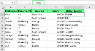
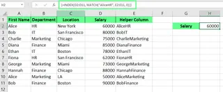
This helper column simplifies my INDEX MATCH formula. Instead of a complex array formula, I can reference the helper column with a much simpler approach:

=INDEX(D2:D11, MATCH("AliceHR", E2:E11, 0))

Method 2: Use an array formula

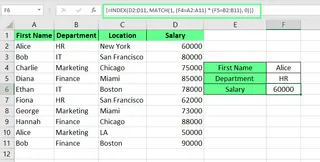
If you prefer not to add extra columns to your sheet, you can use an array formula to handle multiple criteria directly. For example, here’s how I find Alice’s Salary in the HR department without a helper column.

I use the following formula:

=INDEX(D2:D11, MATCH(1, (F4=A2:A11) * (F5=B2:B11), 0))

• (F4=A2:A11) checks for "Alice" in the name column.
• (F5=B2:B11) checks for "HR" in the department column.
• The * operator ensures that MATCH only finds a row where both conditions are TRUE.

Important: In older versions of Excel, you must press Ctrl+Shift+Enter to confirm this as an array formula. Excel will automatically add curly braces {} around it. In newer versions with dynamic arrays, you can just press Enter.

A Simpler, Faster Way: Multi-Criteria Lookups with AI

While array formulas are powerful, they can be complex to write and difficult to debug. This is where an AI tool like Excelmatic changes the game.

Excelmatic is an Excel AI Agent that understands plain language. Instead of building a formula, you just ask a question.

To solve the same problem—finding Alice's salary in the HR department—the process with Excelmatic would be:

1. Upload your Excel file to the Excelmatic platform.
2. Ask your question in the chat interface, just as you would ask a colleague:

   What is the salary for the employee named Alice in the HR department?

Excelmatic instantly scans your data, understands the multiple criteria ("Alice" and "HR"), performs the lookup, and gives you the answer.

The Contrast is Clear:

• INDEX MATCH Array Formula: =INDEX(D2:D11, MATCH(1, ("Alice"=A2:A11) * ("HR"=B2:B11), 0))
  • Requires knowledge of INDEX, MATCH, array syntax, and logical operators.
  • Prone to errors if ranges are incorrect or you forget Ctrl+Shift+Enter.
• Excelmatic: "What is the salary for Alice in HR?"
  • Requires no formula knowledge.
  • Intuitive, fast, and error-free.

This AI-driven approach lets you focus on the question you want to answer, not on the technicalities of how to build the formula.

Advanced Uses for INDEX MATCH with Multiple Criteria

You can do even more with INDEX MATCH, but as we'll see, these complex scenarios also become remarkably simple with an AI assistant.

Nested INDEX MATCH for complex lookups

Sometimes, you need to match criteria for both the row and the column. For example, in this dataset showing sales by product category across different regions, a standard lookup won't work.

I want to find furniture sales in the East. To do this, I need to match "Furniture" in the rows and "East" in the columns. This requires a nested INDEX MATCH formula:

=INDEX(B2:D4, MATCH(D6, A2:A4, 0), MATCH(D7, B1:D1, 0))

Here’s how it works:

• The main INDEX() function looks in the data range B2:D4.
• The first MATCH(D6, A2:A4, 0) finds the row number for "Furniture".
• The second MATCH(D7, B1:D1, 0) finds the column number for "East".

INDEX then returns the value at the intersection of that row and column: 450.

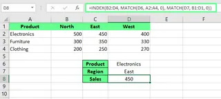
While effective, this formula is even more complex. With Excelmatic, the request is again just a simple question:

What were the furniture sales in the East region?

The AI handles the two-dimensional lookup automatically, saving you from building and debugging a nested formula.

Common Challenges and Troubleshooting

When I started using INDEX MATCH, I ran into several errors. Here’s a look at them and how to solve them—and how an AI approach helps you avoid them altogether.

Handle errors in INDEX MATCH formulas

Errors like #N/A and #VALUE! are common.

• The #N/A error occurs when the MATCH() function can’t find the lookup value. This could be due to a typo, extra spaces (which you can fix with the TRIM() function), or referencing the wrong range.
• The #VALUE! error often appears in a multi-criteria array formula if you forget to press Ctrl+Shift+Enter (in older Excel versions).

The AI Advantage in Troubleshooting

With a tool like Excelmatic, these formula-specific errors disappear. You don't have to debug #N/A, #VALUE!, or #REF! errors because you're not writing the formulas. If the tool can't find the data, it will tell you in plain language (e.g., "I could not find 'Alice' in the dataset") instead of showing a cryptic error code. This makes the entire process of data analysis more forgiving and accessible.

Final Thoughts

Mastering INDEX MATCH is a rite of passage for any serious Excel user. It gives you the power to perform flexible, robust lookups that go far beyond VLOOKUP. Understanding how to build array formulas and nested lookups is a valuable skill that deepens your understanding of how Excel works.

However, the goal of data analysis is to get insights, not to spend hours writing and debugging formulas. Modern AI tools like Excelmatic represent the next evolution in spreadsheet productivity. They allow you to get straight to the answer by simply asking a question.

Ready to transform how you work with Excel data? Try Excelmatic today and experience the power of AI-driven multi-criteria lookups. Simply describe what you need in plain language and let Excelmatic handle all the technical complexity - no formulas to learn, no errors to debug, just instant insights that drive your business decisions forward.

My advice? Learn INDEX MATCH to understand the logic. But for your day-to-day work, embrace the speed and simplicity of AI. Let the machine handle the syntax so you can focus on what the data is telling you.

INDEX MATCH FAQs

How do I handle INDEX MATCH case sensitivity?

By default, INDEX MATCH is not case-sensitive. To make it case-sensitive, you need to combine it with the EXACT function in an array formula:

=INDEX(return_range, MATCH(TRUE, EXACT(lookup_value, lookup_range), 0))

Remember to press Ctrl+Shift+Enter.

How do I handle errors in INDEX MATCH formulas?

Wrap your formula with the IFERROR function to return a custom message instead of an error:

=IFERROR(INDEX(..., MATCH(...)), "Not Found")

What is the difference between using INDEX MATCH and XLOOKUP() for multiple criteria?

XLOOKUP() is a newer, more user-friendly function in Excel that can replace INDEX MATCH for many lookups. For multiple criteria, XLOOKUP is generally simpler than an INDEX MATCH array formula. However, both still require you to learn and write specific formula syntax. An AI tool like Excelmatic is a step beyond both, removing the need to write formulas at all and relying on natural language instead.