Key Takeaways:
- Traditional Excel lookup methods like VLOOKUP and INDEX MATCH require technical knowledge and are prone to errors when columns change
- Excelmatic eliminates formula complexity by letting you perform data lookups using simple language commands
- Compared to traditional methods, Excelmatic handles complex lookup requirements automatically without worrying about column positions or syntax errors
- For business professionals, adopting AI tools means faster data insights and more time for analysis rather than technical implementation
When looking up data in Excel, many people first think of VLOOKUP(). But if you're pursuing higher flexibility and efficiency, the INDEX MATCH combination function is undoubtedly a better choice. It combines the INDEX() and MATCH() functions to provide a more powerful way of data lookup.
This guide will detail the usage of INDEX() and MATCH(), show how they work together, and compare them with traditional methods and modern AI tools. Whether you're an Excel expert or a beginner hoping to simplify your workflow, you'll find the most suitable solution here.
What is INDEX MATCH in Excel?
INDEX MATCH is short for the nested function combination INDEX(MATCH()). To understand its power, we first need to understand these two functions separately.
INDEX() Function
The INDEX() function can return a value or reference to a value from a specified position in a range or table. It has two forms: array form and reference form.
Array Form
Use the array form when working with fixed tables or arrays. INDEX() extracts the corresponding value based on the row and column numbers you specify. Its syntax is:
INDEX(array, row_num, [column_num])
Parameter explanation:
array(required): The cell range or value array you want to operate on.row_num(required): The row number from which you want to return a value.column_num(optional): The column number from which you want to return a value.
You need to specify at least one of row_num or column_num for Excel to locate the value.
Note when using this syntax:
- If the array has only one row or column, you can omit
row_numorcolumn_num. - If both
row_numandcolumn_numare provided,INDEXreturns the value at their intersection. - If you set
row_numorcolumn_numto0, Excel returns the entire column or row (you need to enter it as an array formula to see the result).
Reference Form
Use the reference form when you need to handle multiple ranges and specify lookup areas.
Its syntax is:
INDEX(reference, row_num, [column_num], [area_num])
Parameter explanation:
reference(required): A reference to one or more cell ranges.row_num(required): The row number within the selected range.column_num(optional): The column number within the selected range.area_num(optional): Whenreferencecontains multiple areas, specifies which area to use.
Additional considerations:
- If
area_numis omitted, Excel uses the first area by default. - In this form, referenced areas cannot come from different worksheets, otherwise it will cause an error.
- If both row and column numbers are omitted, the function returns the entire specified area.
MATCH() Function
The MATCH() function helps you find the position of a specific value in a row or column. It returns not the value itself, but the relative position of that value in the list.
Its syntax is:
MATCH(lookup_value, lookup_array, [match_type])
Parameter explanation:
lookup_value(required): The value you want to find.lookup_array(required): The cell range Excel will search.match_type(optional): Defines how Excel matches. Default value is1.1: Finds the largest value less than or equal tolookup_value(requires array to be in ascending order).0: Finds exact match (no sorting required).-1: Finds the smallest value greater than or equal tolookup_value(requires array to be in descending order).
The MATCH function is not case-sensitive. If you want to use wildcards (like * or ?) in text, make sure to set match_type to 0, as only this mode supports wildcard searches.
How Do INDEX() and MATCH() Work Together?
Combining MATCH() with INDEX() is one of its most common uses. MATCH() is responsible for finding the position of the value, while INDEX() extracts the corresponding value based on that position.
By nesting MATCH() within INDEX(), you can build a dynamic and powerful formula that is less prone to errors even if rows or columns are added or moved later.
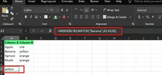
For example, in a sample dataset, if I want to find the value in column B that corresponds to "Banana" in column A, I can use the following INDEX MATCH formula:
=INDEX(B2:B5, MATCH("Banana", A2:A5, 0))
Here, MATCH("Banana", A2:A5, 0) first finds the position of "Banana" in column A (i.e., row 2), then INDEX(B2:B5, ...) returns the value in the same row of column B based on this position.
A Simpler Alternative: Using AI Assistant

Although INDEX MATCH is powerful, writing and understanding it requires some learning. For users pursuing higher efficiency, there's a more intuitive approach.
Excelmatic, an Excel AI assistant, allows you to perform data lookups using natural language. You don't need to write any formulas - just upload your file and ask questions in any language.
For the example above, you just need to ask Excelmatic:
What's the value in column B that corresponds to 'Banana' in column A?
Excelmatic will immediately understand your request and provide the correct answer. This approach is not only faster but also completely avoids problems caused by formula syntax errors.

Choose Your Lookup Method: Formula vs. AI
INDEX MATCH can accomplish tasks that VLOOKUP cannot handle. But now, we have more choices. Let's compare VLOOKUP, INDEX MATCH, and AI tools.
VLOOKUP vs. INDEX MATCH: Traditional Methods Face-off
1. Column Flexibility and Data Integrity
The biggest disadvantage of VLOOKUP is its reliance on fixed column numbers. If you insert or move columns, the formula will likely fail.
For example, this VLOOKUP formula:
=VLOOKUP("Apple", A2:C5, 2, FALSE)
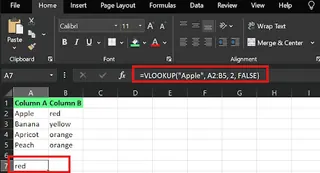
If a new column is inserted between columns A and B, the original third column moves, and the formula returns incorrect results.
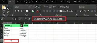
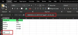
INDEX MATCH avoids this problem by using defined ranges instead of hard-coded column numbers:
=INDEX(B2:B5, MATCH("Apple", A2:A5, 0))
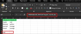
Even if columns are rearranged, this formula remains effective, making it more reliable and easier to maintain. This is the magic of INDEX MATCH.
2. Lookup Direction and Versatility
VLOOKUP can only look from left to right, meaning your lookup column must be the first column in the data range.
INDEX MATCH has no such limitation. You can look in any direction: left, right, up, down. It also supports horizontal lookups, giving you more control over data organization.
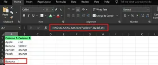
For example, looking from right to left (finding the fruit name based on the color "yellow"):
=INDEX(A2:A5, MATCH(“yellow”, B2:B5,0))
Formula vs. AI: A New Way of Data Lookup
INDEX MATCH is undoubtedly superior to VLOOKUP, but compared to AI tools like Excelmatic, it still requires manual construction and debugging.
| Feature | VLOOKUP |
INDEX MATCH |
Excelmatic (AI) |
|---|---|---|---|
| Ease of Use | Medium | Difficult | Extremely Easy (natural language) |
| Lookup Direction | Left to right only | Any direction | Any direction (AI automatically understands) |
| Column Changes | Error-prone | Robust | Extremely robust (doesn't rely on column positions) |
| Performance | Slow for large tables | Faster | Instant (cloud processing) |
| Learning Curve | Shorter | Longer | Almost zero |
The core advantage of AI tools lies in process simplification and error reduction. You no longer need to memorize complex function syntax or worry about #REF! errors caused by column changes. The AI assistant understands your data and your questions, providing answers directly.
When to use INDEX MATCH:
- You're working with large, dynamic data models where columns are frequently added or deleted.
- You need to look left or perform horizontal lookups.
- You're an experienced Excel user who enjoys complete control over formulas.
When to use AI tools (like Excelmatic):
- You need quick answers from data and don't want to spend time writing or debugging formulas.
- You're unfamiliar with Excel formulas, or team members have varying Excel skill levels.
- Your task is exploratory data analysis requiring frequent questions.
How to Use INDEX MATCH: Step-by-Step Guide
Suppose you have two columns: Fruits and Sales. You want to find the sales for "Apple".
Enter the following INDEX MATCH combination formula and press Enter:
=INDEX(B2:B6, MATCH("Apple", A2:A6, 0))
Here, MATCH("Apple", A2:A6, 0) finds the position of "Apple" in the fruit list. Then, INDEX(B2:B6, ...) uses that position to return the corresponding value in the sales column.
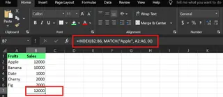
The formula returns 12000, which is exactly Apple's sales.
Avoiding INDEX MATCH Errors
Although INDEX MATCH is powerful, it can still return errors if not set up correctly. Here's how to troubleshoot common problems.
#N/A Error and Solutions
The #N/A error means Excel cannot find the value you're looking for. Common causes include:
- Spelling errors, extra spaces, or text format mismatches.
- The value doesn't exist in the lookup range.
- Incorrect
match_typesetting (e.g., using1instead of0when exact match is needed).
Solutions:
- Use the
TRIM()function to remove extra spaces:=MATCH(TRIM("Apple "), A2:A6, 0) - Use the
IFERROR()function to provide a fallback value:=IFERROR(INDEX(B2:B6, MATCH("Apple", A2:A6, 0)), "Not found")
#REF! Error
The #REF! error typically points to an invalid reference, possibly because:
- The ranges for
INDEX()andMATCH()functions don't match in size. - Rows or columns that the formula depends on have been deleted.
Solutions:
- Ensure the ranges for
INDEX()andMATCH()are the same size. - Use absolute references (like
$A$2:$A$6) to lock ranges and prevent formula errors during copy-paste.
How AI Avoids These Errors?
Using AI tools like Excelmatic, you can basically say goodbye to the above formula errors.
- Goodbye
#N/A: You just ask questions in natural language. AI handles minor spelling differences better, and if it can't find data, it gives clear prompts (like "No relevant data found for 'Apple'") instead of confusing error codes. - Goodbye
#REF!: Since there are no manually set cell references, there's no risk of reference failure. No matter how you move, add, or delete columns, AI can understand your data structure through column headers (like "Sales").
Final Thoughts
If you've been relying on VLOOKUP, it's time to switch to a more stable and powerful method. You can start by trying INDEX MATCH for some simple lookups in a copy of your work file. Once you experience its advantages in handling column changes and complex lookups, you might never go back.
However, technological advancements provide us with simpler choices. For those who want to spend time analyzing results rather than writing formulas, AI tools like Excelmatic are becoming the new standard. They free you from complex syntax, allowing you to converse with your data in the most natural way.
Ultimately, choosing between INDEX MATCH and AI tools depends on your specific needs, Excel proficiency, and your pursuit of work efficiency.
Ready to transform your Excel workflow? Try Excelmatic today and experience the power of AI-driven data analysis. Simply describe what you need in plain language and let Excelmatic handle all the technical complexity - no formulas to learn, no errors to debug, just instant insights that drive your business decisions forward.
XLOOKUP() vs. INDEX MATCH: Which is Better?
It depends on your usage scenario. XLOOKUP() is a new function introduced in Excel 365 and later versions. It's designed to be simpler than INDEX MATCH and in some cases (like using binary search mode) computes faster. But INDEX MATCH is available in all modern Excel versions and has better compatibility.

