A Smarter Way to Combine VLOOKUP and IF in Excel

If you manage large datasets in Excel, you know how challenging it is to organize and analyze them efficiently. A classic solution is to nest the VLOOKUP() function inside an IF() statement to create dynamic lookups based on specific conditions. This powerful combination allows you to look up different tables based on a condition and handle errors more gracefully.

VLOOKUP() finds specific data points within a table, and IF() statements allow you to make conditional decisions based on that data. While mastering these functions is a valuable skill, what if there was a faster, more intuitive way?

In this article, we'll explore both the traditional method of combining these functions and introduce a modern AI-powered approach. You will learn how to leverage the power of both of these functions together to perform conditional lookups, and we will also see how an AI agent like Excelmatic can achieve the same results with simple language commands, saving you from complex, nested formulas.

The Quick Answer: Two Ways to Combine VLOOKUP and IF

The Traditional Formula Method

To create a conditional lookup, you start with an IF() statement and use VLOOKUP() inside it to return different results based on a condition. For example, the following formula checks if a product is in stock based on its quantity:

=IF(VLOOKUP(C2, $A$2:$B$6, 2, FALSE) > 0, "In Stock", "Out of Stock")

The AI-Powered Alternative: Excelmatic

With an AI agent like Excelmatic, you can skip the formula syntax entirely. Simply upload your file and state your request in plain language:

For each product, check if its quantity is greater than 0. If it is, show 'In Stock', otherwise show 'Out of Stock'.

Excelmatic handles the logic and returns the results instantly, without you needing to write or debug a single formula.

Understanding VLOOKUP() and IF() Statements in Excel

VLOOKUP() helps you find data in a table, while IF() statements let you decide based on that data. Together, they are a cornerstone of data analysis in spreadsheets. Let’s look at each function separately before combining them.

What is VLOOKUP() in Excel?

VLOOKUP() searches for a specific value in the first column of a range and returns a value from another column in the same row. Here’s the syntax:

=VLOOKUP(search_key, range, index, is_sorted)

Let’s break down this syntax:

• search_key is the value you want to search for.
• range defines the cell range containing the data. The first column in this range must contain the search_key.
• index is the column number in the range from which you want to retrieve a value (the first column is 1, the second is 2, etc.).
• is_sorted is a logical value (TRUE for an approximate match, FALSE for an exact match). For most use cases, FALSE is recommended to prevent unexpected results.

Let’s understand with an example. Here I have a list of products with their IDs and prices. I want to find the prices for specific products based on their name.

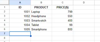
To find the price of a "Tablet", I would enter "Tablet" in a cell (e.g., E2) and then use the following formula:

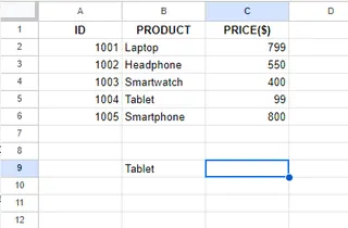
The formula would be =VLOOKUP(E2, A2:B6, 2, FALSE).

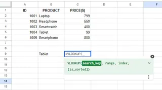
Let's break down the steps:

1. search_key: Select the cell containing "Tablet".
2. range: Select the entire data table (A2:B6).
3. index: Enter 2, as the price is in the second column.
4. is_sorted: Enter FALSE for an exact match.

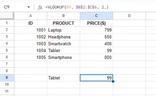
As you can see, VLOOKUP() successfully retrieves the price.

What is IF() in Excel?

IF() statements check if a condition is met and return one value if TRUE and another value if FALSE. Here is the syntax:

=IF(logical_test, [value_if_true], [value_if_false])

Let’s look at the key parts:

• Logical_test is the condition you want to check.
• Value_if_true is the value returned if the condition is TRUE.
• Value_if_false is the value returned if the condition is FALSE.

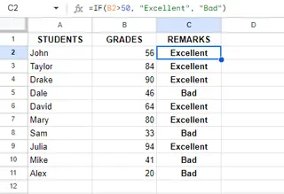
For example, to assign "Excellent" or "Bad" remarks based on student grades being above or below 50:

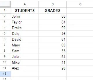
The formula in the remarks column would be =IF(B2>50, "Excellent", "Bad"). By dragging this formula down, you can quickly assign remarks to all students.

Ways to Combine VLOOKUP() with IF() in Excel

Now let's explore practical examples of how these functions work together and see how an AI alternative simplifies the process.

Conditional Lookups

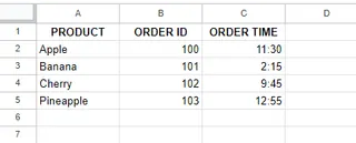
Let's say we have a list of product orders and want to see if a product was ordered before or after noon (12:00 PM).

The Traditional Formula Method:

You would use this complex nested formula:

=IF(VLOOKUP(A3, A2:C5, 3, FALSE) < TIME(12, 0, 0), "Ordered Before Noon", "Ordered After Noon")

Here, VLOOKUP finds the order time, and IF checks if it's before 12:00 PM.

The AI-Powered Alternative: Using Excelmatic

Forget the TIME() function and nested lookups. Just upload your sheet and ask:

For each product, check if the Order Time is before 12:00 PM. If it is, return 'Ordered Before Noon', otherwise return 'Ordered After Noon'.

Excelmatic interprets your request and generates the result, simplifying the task immensely.

Error Handling

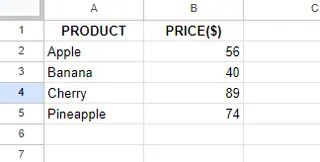
A common issue with VLOOKUP is the ugly #N/A error when a value isn't found. You can use IF combined with ISNA (or the simpler IFERROR) to show a custom message.

The Traditional Formula Method:

To find the price of a product in cell B7 and show "Product Not Found" on error, the formula is:

=IF(ISNA(VLOOKUP(B7, $A$2:$B$5, 2, FALSE)), "Product Not Found", VLOOKUP(B7, $A$2:$B$5, 2, FALSE))

This formula is long because you have to write the VLOOKUP part twice.

The AI-Powered Alternative: Using Excelmatic

Natural language is perfect for handling "if-then-else" logic. Simply ask:

Find the price for the product in cell B7. If the product doesn't exist in the table, just say 'Product Not Found'.

Excelmatic understands the conditional error handling and provides a clean output without you needing to know ISNA or IFERROR.

Dynamic Column Indexing

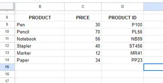
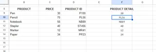
Sometimes, you want to retrieve data from different columns based on a condition. For example, look up a product's stock quantity if its price is above $50, otherwise, look up its ID.

The Traditional Formula Method:

This requires a very complex formula with three VLOOKUP functions:

=IF(VLOOKUP(B9, $B$9:$D$14, 2, FALSE) > 50, VLOOKUP(B9, $B$9:$D$14, 3, FALSE), VLOOKUP(B9, $B$9:$D$14, 2, FALSE))

This formula first looks up the price to check the condition, then performs another lookup to return either the stock (column 3) or the price again (column 2). It's powerful but difficult to read and maintain.

The AI-Powered Alternative: Using Excelmatic

Describe the logic directly:

For each product, if its price is greater than 50, show its stock quantity. Otherwise, show its price.

This simple instruction replaces a convoluted formula, making your analysis faster and less prone to errors.

Advanced Techniques: Multiple Criteria and Calculations

The combination of IF and VLOOKUP can handle even more advanced scenarios.

Combining Multiple Criteria

Let's say you want to check if a customer is eligible for a loyalty program, which requires a total purchase of at least $500 AND a "Gold" membership status.

The Traditional Formula Method:

Here, you need to add the AND function inside your IF statement:

=IF(AND(VLOOKUP(B2, $B$2:$D$11, 2, FALSE) >= 500, VLOOKUP(B2, $B$2:$D$11, 3, FALSE) = "Gold"), "Eligible", "Not Eligible")

This formula checks two separate conditions before returning a result.

The AI-Powered Alternative: Using Excelmatic

The logic is much clearer in plain language:

Create a new column called 'Eligibility'. A customer is 'Eligible' if their 'TOTAL PURCHASE ($)' is 500 or more and their 'MEMBERSHIP STATUS' is 'Gold'. Otherwise, they are 'Not Eligible'.

Using VLOOKUP() with IF() for Calculations

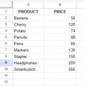
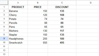
You can also perform calculations based on a lookup. For instance, apply a 10% discount (multiplying by 0.9) to products with a price over $100.

The Traditional Formula Method:

=IF(VLOOKUP(A2, $A$2:$B$10, 2, FALSE) > 100, VLOOKUP(A2, $A$2:$B$10, 2, FALSE) * 0.9, VLOOKUP(A2, $A$2:$B$10, 2, FALSE))

This formula is inefficient as it performs the same VLOOKUP up to three times.

The AI-Powered Alternative: Using Excelmatic

Simply describe the calculation you want:

Create a 'DISCOUNT' column. If a product's price is over $100, calculate the price with a 10% discount. Otherwise, show the original price.

Final Thoughts

Combining VLOOKUP() with IF() statements is a testament to Excel's power, allowing for sophisticated, dynamic, and error-resistant spreadsheets. Mastering these formulas is a valuable skill for any data professional.

However, the landscape of data analysis is evolving. AI-powered tools like Excelmatic offer a compelling alternative that prioritizes speed and ease of use. By allowing you to use plain language, they remove the steep learning curve of complex nested formulas, reduce the chance of syntax errors, and ultimately let you focus on the insights, not the process.

Whether you choose to master the formulas or leverage an AI assistant, the goal remains the same: to turn raw data into meaningful information. The best approach is often a hybrid one—knowing the fundamentals of Excel while embracing new tools that make your work faster and smarter.

Ready to revolutionize how you handle complex Excel formulas? Try Excelmatic today and experience instant conditional lookups with just a simple command.