The Ultimate Guide to Removing Duplicates in Excel

Dealing with duplicate data in Excel can be an annoying process. Fortunately, modern Excel has a powerful tool for the job: the UNIQUE() function. It’s a simple formula, but it’s a must-know for extracting distinct entries from any range. But what if you could achieve the same result without writing any formulas at all?

In this article, you will see clear examples of how to use the UNIQUE() function. We'll also introduce an AI-powered alternative, Excelmatic, to show you how you can get the same results using just plain language. Let's compare these two powerful approaches.

Method 1: The Formula Approach with Excel's UNIQUE() Function

Let’s start with Excel’s built-in solution. The UNIQUE() function returns a list of unique values from a range or array, automatically filling as many cells as needed. This is known as a dynamic array. This makes it great for instantly stripping duplicates from a column or generating fresh lists for dropdown menus or reports.

A quick heads up: UNIQUE() is available only in Excel for Microsoft 365, Excel 2021, and Excel for the web. If you’re using an older version, you'll need an alternative, which we'll touch on later.

Excel UNIQUE() Function Syntax

Here's the syntax for the UNIQUE() function:

=UNIQUE(array, [by_col], [exactly_once])

Here’s what each argument means:

• array: The range or array from which you want to extract unique values.
• by_col (optional): Set this to TRUE to compare columns instead of rows. Most of the time, you’ll leave it blank or set to FALSE.
• exactly_once (optional): Set to TRUE if you want only values that appear once in the source array. By default (FALSE), you’ll get all distinct values, even if they appear more than once.

Now, let's see it in action.

Excel UNIQUE() for Values in a List

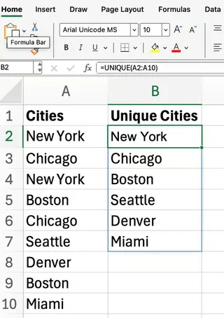
Suppose you have a list of cities in column A (A2 to A10), and some cities are listed more than once. To pull out just the unique city names, enter this:

=UNIQUE(A2:A10)

Excel will “spill” the unique city names down the column. As long as the function is there, your list will update as your source data changes—a big time-saver.

Excel UNIQUE() Across Multiple Columns

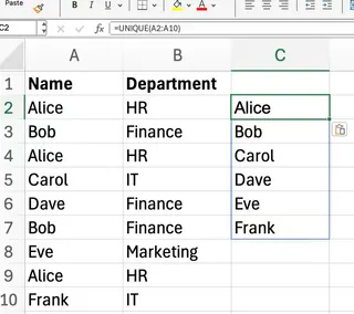
What if your data spans more than one column? Let’s say you have a two-column table (A2:B10) with names and departments, and you want to see each unique name/department pair only once.

=UNIQUE(A2:B10)

With this formula, Excel returns each unique combination of name and department, eliminating duplicate rows. If you only care about unique names, you can point UNIQUE() directly to just the name column:

=UNIQUE(A2:A10)

Excel UNIQUE() to Show Values That Appear Exactly Once

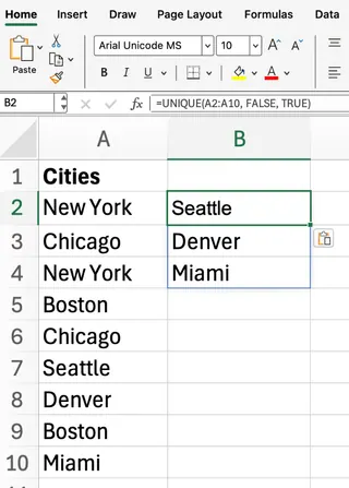
By default, UNIQUE() gives you all distinct values. But you can also use it to filter for values that appear exactly once. For this, we will use the exactly_once argument.

=UNIQUE(A2:A10, FALSE, TRUE)

This formula returns only the values from A2:A10 that occur a single time. Notice how New York, Chicago, and Boston are not included.

Excel UNIQUE() to Get Unique Columns Instead of Rows

So far, we’ve focused on extracting unique rows, but UNIQUE() can also find unique columns. If you set by_col to TRUE, Excel compares columns and returns the distinct ones. This is less common, but useful in certain scenarios.

=UNIQUE(A1:F1, TRUE)

Here, Excel checks each column within the range and gives you only the columns that are different from one another.

Method 2: The AI-Powered Way with Excelmatic

The UNIQUE() function is powerful, but you still need to remember the syntax and its arguments. Excelmatic, an Excel AI Agent, offers a more intuitive path. You simply upload your file and describe what you need in plain language.

Let's see how Excelmatic handles the same tasks.

• To get a list of unique cities: Instead of writing =UNIQUE(A2:A10), you would upload your file to Excelmatic and ask:

  Give me a list of unique cities from column A.

• To find unique name/department pairs: Instead of =UNIQUE(A2:B10), your request would be:

  Show me each unique combination of name and department.

• To find values that appear only once: Rather than remembering the exactly_once argument with =UNIQUE(A2:A10, FALSE, TRUE), you can just ask:

  List all cities that appear only once.

The key advantage is simplicity. There are no formulas to write or arguments to remember. You state your goal, and the AI handles the execution.

Combining Functions: The Ultimate Test

The true power of these tools shines when you combine operations.

With Formulas: UNIQUE() + SORT() + FILTER()

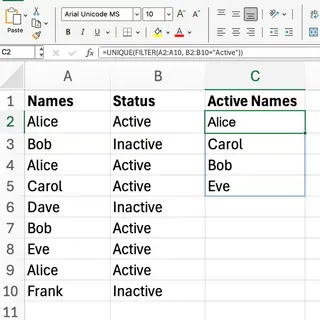
To get a sorted list of unique values that meet a condition (e.g., only for "Active" entries), you need to nest multiple functions:

=SORT(UNIQUE(FILTER(A2:A10, B2:B10="Active")))

This formula first FILTERs for "Active" rows, then finds the UNIQUE items, and finally SORTs them alphabetically. It's efficient, but complex to write.

With Excelmatic: A Single Command

With Excelmatic, you can accomplish the same multi-step task with one simple request:

Give me a sorted list of unique items where the status in column B is Active.

Excelmatic processes the entire request—filtering, de-duping, and sorting—in one go, delivering the final, clean list instantly.

Which Method is Right for You?

Use the UNIQUE() function if:

• You are comfortable with Excel formulas and prefer to work directly within your worksheet.
• You need the list of unique values to be dynamic and update automatically inside your spreadsheet as the source data changes.
• You have a modern version of Excel (Microsoft 365 or 2021).

Use Excelmatic if:

• You want the fastest, most intuitive way to get an answer without writing formulas.
• You need to perform complex, multi-step data cleaning tasks quickly.
• You prefer to describe your needs in plain English and let an AI agent do the heavy lifting.

For users of older Excel versions without UNIQUE(), traditional methods involved complex IFERROR(INDEX(...)) array formulas or using the "Remove Duplicates" tool and PivotTables. Compared to these, both UNIQUE() and Excelmatic represent a massive leap in efficiency.

Common Issues with UNIQUE()

If you stick with the formula approach, watch out for these common issues:

• The results “spill” into as many rows or columns as needed. If you type in any of these cells, you’ll get a #SPILL! error—so keep those cells clear.
• UNIQUE() is case-insensitive, treating “Apple” and “apple” as the same.
• The output updates automatically when your source data changes, which is a feature, not a bug!

Conclusion

Whether you're cleaning data, creating dropdown lists, or summarizing information, removing duplicates is a fundamental Excel task.

Excel's UNIQUE() function is a fantastic tool for anyone who loves working with formulas and wants dynamic, in-sheet results. However, for market, sales, and operations professionals who prioritize speed and simplicity, AI tools like Excelmatic offer a revolutionary alternative. By allowing you to use natural language, they remove the learning curve of functions and syntax, letting you focus on the insights and strategic decisions, not the technical process.

Ready to transform how you work with Excel data? Try Excelmatic today and experience the power of AI-driven data cleaning - no formulas, no complexity, just results.