Key Takeaways:
- Data filtering is essential for business analysis, reporting, and dashboard creation, but traditional Excel Slicers require complex setup and technical knowledge
- Excelmatic's AI approach eliminates the need for Slicer configuration by letting you filter data instantly using simple language commands
- Compared to Slicers, Excelmatic handles complex multi-table filtering and ad-hoc analysis without any setup, formatting, or compatibility issues
- For business users, adopting AI tools means faster insights and more time for decision-making rather than technical dashboard building
Excel Slicers simplify data filtering and make visualizations much easier to understand. You don’t have to run through dropdown menus to find specific data because slicers let you interact with it in a visually clear way. While slicers are a huge leap forward from traditional filters, modern AI tools now offer an even faster path to the same insights.
In this article, I’ll show you how slicers work, their advantages, and even some advanced techniques. I'll also introduce a powerful AI-driven alternative, Excelmatic, and compare the two approaches. Along the way, I’ll share examples to help you see how you can save time and make your analysis more efficient, no matter which method you choose.
What is an Excel Slicer?
The slicer is a filtering tool that was introduced in Excel 2010. Unlike dropdown menus, it gives you interactive buttons to filter your PivotTables and tables. You can narrow down your data with a single click and the best part is, you’ll always know which filters are active.
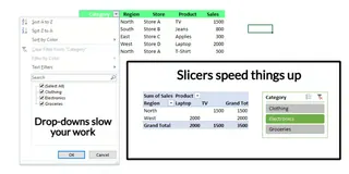
Drop-down menus versus Excel slicers. Image by Author.
Most of the time, I use slicers to track my monthly projects and isolate specific categories in a report. Instead of running through dropdown menus, I just click a button and instantly see the data I need — it’s that simple.
Slicers help me focus on what’s important without getting distracted by everything else. That’s why, for me, the biggest win is how they cut through the noise. They’ve also become a go-to when I’m building dashboards because they add a polished and professional touch.
So, if you haven’t tried slicers yet, they are a fantastic tool that is as valuable for beginners as it is for experts.
How to Insert an Excel Slicer
Now that you know what slicers are, I will walk you through how to add them to your Excel tables, PivotTables, and PivotCharts. It’s a straightforward process, and I’ll share a few tips to make it even more effective.
Add slicers to a PivotTable
Here’s how you can add a slicer to a PivotTable:
- Click anywhere on your PivotTable.
- Go to the Insert tab, find the Filters group, and click Slicer. Alternatively, you can head over to the Analyze tab and, under the Filter group, select Insert Slicer.
- A window will pop up showing all the fields in your PivotTable. Check the boxes next to the ones you want to filter with a slicer.
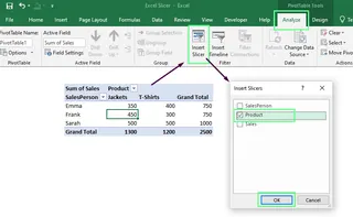
Insert a slicer into the PivoTable. Image by Author.
- Click OK, and the slicer will appear on your sheet.

Slicer activated. Image by Author.
Add slicers to a PivotChart
Here’s how you can add a slicer to a PivotChart:
- Click anywhere on your PivotChart.
- Go to the Analyze tab. From the Filter group, click Insert Slicer.
- Check the fields you want to filter. Then, Click OK.
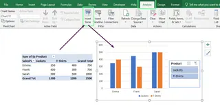
Insert a slicer into the PivotCharts. Image by Author.
When I use slicers, I hide the chart’s filter buttons because they clutter the view. To clean things up, I even resize the chart area to fit the slicer inside. It keeps everything neat and easy to work with.
As a note, if your PivotTable and PivotChart are connected, the same slicer will work for both.
Add slicers to an Excel table
If you work with a regular table in Excel (and not PivotTables), slicers are still an option. Here’s how to add them:
- Click anywhere inside your table.
- Go to the Insert tab, find the Filters group, and click Slicer.
- In the window that pops up, check the boxes for the columns you want to filter.
- Click OK, and the slicer will appear and be ready to use.
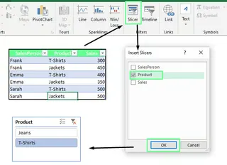
Insert a slicer into the table. Image by Author.
Now, a quick tip: When you choose fields for a slicer, think about what will make your data easier to handle. For example, slicing by fields like Region, Month, or Salesperson would work best if you analyze sales data. So, focus on the dimensions that matter most to your analysis to quickly find the important insights.
The AI Alternative: Instant Filtering with Excelmatic
While slicers are powerful, they require a multi-step setup. For those who want answers instantly without building interactive components, an AI Excel Agent like Excelmatic offers a revolutionary approach.
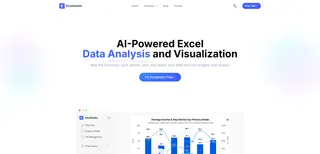
With Excelmatic, the process is much simpler:
- Upload your Excel file.
- Ask your question in plain language.
For example, instead of clicking through Insert > Slicer > Select Field > OK, you can simply type: "Filter the sales data to show only the 'North' region and 'Electronics' category." Excelmatic analyzes your request and provides the filtered data or a chart immediately. This conversational method bypasses the entire setup process, making data filtering faster and more intuitive.
How to Customize the Excel Slicer Appearance
For those who build dashboards, visual appeal is key. Let me show you how you can tweak your slicer appearance to match your workbook style.
Change the slicer style
Click on your slicer to bring up the Slicer Tools tab. Under this tab, go to the Options section and check out the Slicer Styles group. Here, you’ll see several built-in styles — pick one you like.

Slicer styles. Image by Author.
If you don't like any of the built-in styles, you can create one. Click the drop-down (More) button and select New Slicer Style. From here, you can build a custom style that matches your spreadsheet theme.
For example, if I’m working with a dashboard that has a cool blue theme, I’ll create slicer colors in complementary shades of blue. It would make everything look more cohesive.
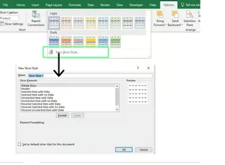
Build your own slicer style. Image by Author.
Adjust slicer settings
If you want to tweak your slicer further, right-click on it and select Slicer Settings. From here, you can make a lot of adjustments. For example, you can hide the slicer header if it doesn’t add value or hide items without data to make it look cleaner and more focused.
Although these are minor adjustments, they can make the slicer much more user-friendly.
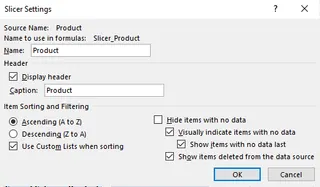
Slicer settings. Image by Author.
Optimize slicer layout
When my slicer has a lot of items, the default single-column view drives me crazy because it requires so much scrolling. To fix that, I click the slicer, go to the Slicer Tools Options tab, and adjust the Columns setting. I usually set it to 2 or 3 columns, depending on the slicer content.
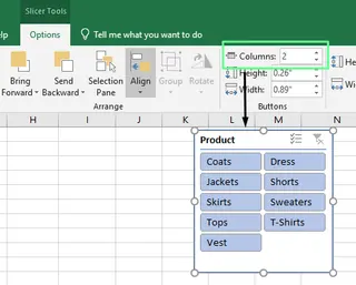
Adjust the columns of the slicer. Image by Author.
I also adjust the button sizes to make everything look balanced. To do so, go to the Slicer Tools Options tab, tweak the height and width settings, or drag the edges of the slicer until they look right. However, I’d recommend keeping the slicer buttons large enough to be easy to click but not so big that they take over the whole sheet.
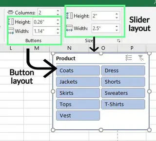
Changing the width and height of the slicer and its button. Image by Author.
Advanced Excel Slicer Techniques
Besides basic filtering, you can create interactive reports and dashboards with Excel slicers. Let me show you some of my favorite tricks for doing that.
Connect slicers to multiple PivotTables
One of the coolest features of slicers is the ability to link a single slicer to multiple PivotTables. This is really helpful when you work with related datasets. It lets you filter all your data at once with a single click — you don’t have to update each table manually. Here’s how I used this technique to analyze student performance data:
- I created all the PivotTables I wanted to link. To keep things manageable, I placed them on the same worksheet.
- Next, I gave each PivotTable a unique name. This made it much easier to identify them when I set up the connections.
- Then, I added a slicer to one of the PivotTables.
- Once the slicer was in place, I selected it, went to the Slicer Tools Options tab, and clicked Report Connections. Alternatively, you can right-click on the slicer and choose Report Connections.
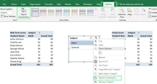
Connect a slicer to multiple PivotTables. Image by Author.
- In the dialog box that popped up, I checked the boxes for the PivotTables I wanted to link to the slicer and clicked OK.
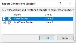
Specify the PivotTables to link. Image by Author.
Now, I can filter this data with a single click to see the students' midterm and final scores. It saves so much time and makes analyzing multiple PivotTables easy.
In contrast, an AI tool like Excelmatic handles this inherently. You can upload multiple related files or use a single file with multiple tables and simply ask a question that spans across them. The AI manages the relationships behind the scenes, delivering a unified answer without any manual Report Connections setup.

Two PivotTables linked with one slicer. Image by Author.
Optimize Excel slicer performance
Slicers can sometimes slow down if you work with large datasets. Here are common issues and the solutions that worked for me:
- Slow performance: If slicers lag, it’s usually because they’re processing too much data. To fix this, filter out data you don’t need or create a summary table with only the important information.
- Multiple slicers for multiple tables: Managing multiple slicers is messy. Instead, connect one slicer to multiple tables using Report Connections.
- Clicking doesn’t filter anything: If a slicer isn’t filtering, it’s likely not linked correctly. Right-click the slicer, select Report Connections, and ensure it’s connected to the right tables.
- Seeing old data in the slicer: Slicers can display items that no longer exist in your data. To fix this, go to Slicer Settings and uncheck Show items deleted from data source.
- Non-updated data: If a slicer isn’t reflecting recent changes, right-click the PivotTable and select Refresh.
- Cluttered slicer layout: To fix a long, single-column slicer, go to Slicer Tools Options and increase the column count.
- Hidden slicer: If you can’t see your slicer, it may be behind other elements. Right-click it and choose Bring to Front.
Excel Slicer vs. Excelmatic: Which Filtering Method is Right for You?
You now have two powerful ways to filter data: the manual, visual approach of Slicers and the conversational, instant approach of an AI agent like Excelmatic. Let’s compare them to see which is best for your needs.
| Feature | Excel Slicer | Excelmatic (AI Agent) |
|---|---|---|
| Setup | Manual: Requires creating a Table/PivotTable, then inserting and configuring the slicer. | Instant: Just upload your file(s). No setup needed. |
| How it Works | Click visual buttons on a pre-defined filter component. | Ask a question in plain language (e.g., "What were the top 5 products in Germany?"). |
| Flexibility | Limited to the fields you create slicers for. Adding new filters requires manual changes. | Unlimited. Filter, sort, and aggregate by any data point in your file, on the fly. |
| Use Case | Building pre-defined, interactive dashboards for others to explore within set parameters. | Fast, ad-hoc data analysis, answering complex questions, and generating insights without manual work. |
| Learning Curve | Moderate. Requires knowledge of Tables, PivotTables, and Slicer settings. | Minimal. If you can ask a question, you can use it. |
When to use each
Let’s say I want to filter all students’ math grades for the fall semester. Here’s how each approach handles it:
- Using Slicers: I’d first set up my data in a table or PivotTable, then insert slicers for "Semester" and "Subject". I'd place them next to my table. With two clicks—one on "Fall" and one on "Math"—I can visually filter the data. This is great for a reusable report that others will use.
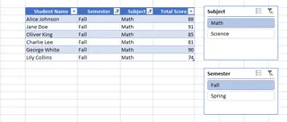
Data filtered using slicers. Image by Author.
- Using Excelmatic: I’d upload the student data file and simply ask, "Show me the math grades for the fall semester." Excelmatic would instantly generate the filtered table or a summary. This is ideal for getting a quick answer without any setup, especially if my next question is completely different, like "What was the average grade in history across all semesters?"
In short, Slicers are the right tool when you need to build a polished, interactive, and user-friendly dashboard for a specific, recurring analysis. But for speed, flexibility, and exploring data with complex, one-off questions, an AI agent like Excelmatic is the more powerful and efficient choice.
Final Thoughts
Excel slicers make it simple and easy to filter data without manual sorting. Personally, I’ve found them invaluable in managing projects and building dashboards. They save time and help me focus.
However, the landscape of data analysis is changing. While slicers are a fantastic manual tool, AI agents like Excelmatic represent the next leap forward. By allowing you to simply ask for what you need, they make data analysis conversational, removing the technical barriers of setup and configuration.
Ready to transform your data filtering experience? Try Excelmatic today and discover how AI-powered analysis can accelerate your business insights.
Excel Slicer FAQs
Can I lock a slicer to prevent users from moving or resizing it?
Yes, you can. To do so, right-click on the slicer and choose Size and Properties. Under the Format Slicer window, open Position and Layout, and check Disable resizing and moving.
Can I insert a slicer without a PivotTable?
Yes, you can, but only if your data is formatted as an Excel table.
Why can't I insert a slicer?
This can happen if your data isn't in a Table or PivotTable, the worksheet is protected, the workbook is shared, or you're using an Excel version older than 2010. Ensure your data is formatted correctly and your workbook settings allow it.
Can an AI tool replace slicers completely?
It depends on the task. For creating static, interactive dashboards for wide distribution, slicers are still excellent. For personal analysis, quick reporting, and exploring data with complex queries, AI tools like Excelmatic are often faster and more powerful.
How do I select multiple buttons in a slicer?
Hold down the Ctrl key while clicking on the slicer buttons, or click the Multi-Select icon in the slicer's header.
How do I disconnect a slicer from a PivotTable or table?
Click the PivotTable, go to Analyze > Filter Connections (or Options > Slicer Connections in Excel 2010), and uncheck the slicer to disconnect.

