Beyond MATCH - Simpler Ways to Find Data Positions in Excel

In this article, I will show what makes Excel's MATCH() function a unique and powerful tool for data lookups. But more importantly, we'll explore how modern AI tools are revolutionizing this task, offering a faster, more intuitive path to the same answers.

What makes MATCH() unique is that, unlike VLOOKUP() or HLOOKUP(), which return actual values, MATCH() gives us the position of a value. This can be extremely useful in many situations, but it often requires writing complex formulas. Let’s see how the traditional method compares to a new, AI-powered approach.

The Quick Answer: Two Ways to Find Data

Finding the position of a value is a common task. Here are two ways to do it: the classic formula-based way and the modern AI-powered way.

The Traditional Way: Using the MATCH() Function

To find the position of a value using the MATCH() function:

• Click on an empty cell where you want the result.
• Type =MATCH(.
• Then write the lookup value in inverted commas (or reference a cell).
• Select the lookup_array.
• Enter the match type (0 for exact match) and hit Enter.

For example, with a list of fruits and their sales in the A2:B6 range, to find the position of "Orange," you would write the following formula and press Enter:

=MATCH(“Orange”, A2:A6, 0)

This will display 4 because "Orange" is the fourth item in the list starting from A2.

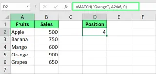Use the MATCH() function. Image by Author.

The AI-Powered Way: Using Excelmatic

With an AI agent like Excelmatic you can skip the formula syntax entirely.

• Upload your Excel file.
• Ask a question in plain language, like: "What is the position of 'Orange' in the first column?"

Excelmatic processes your request and gives you the answer directly, without you needing to remember function names, arguments, or syntax. It's a faster, more intuitive way to get the same result.

Understanding Excel MATCH()

While AI tools offer a shortcut, understanding the MATCH() function is still valuable. There’s more than one way to use it, and how we use it can change what we get from it. Let’s understand this in more detail.

What is the MATCH() function?

The MATCH() function in Excel returns the relative position of a value in a list. Instead of giving the actual value, it tells us where that value is located. This is essential when you need to feed a row or column number into another function, creating dynamic and powerful formulas.

Syntax of the MATCH() function

The syntax of MATCH() is:

MATCH(lookup_value, lookup_array, [match_type])

Here:

• lookup_value is the value we’re looking for in lookup_array.
• lookup_array is the range of cells being searched.
• match_type (optional) tells how to search. 1 (default) finds the largest value less than or equal to the lookup_value (list must be sorted ascending). 0 finds an exact match. And -1 finds the smallest value greater than or equal to the lookup_value (list must be sorted descending).

Key things to know about the MATCH() function

Before you use the MATCH() function, a few small things are worth knowing. They’ll help you avoid mistakes and make things a bit easier:

• MATCH() is not case-sensitive, so "apple," "Apple," and "APPLE" are treated the same.
• If we work with text and set the match_type to 0, we can use wildcards such as an * to represent multiple characters and a ? to represent a single character.
• If MATCH() cannot find your desired value, it will return an #N/A error.

Basic Examples of Using Excel MATCH()

Now that we know what the MATCH() function is and how it works, let's see how we can use it and how an AI tool simplifies the process.

Example 1: Finding the position of a number

Let's say you have a range of numbers in cells A2:A7 and want to find the position of the number 40.

The Formula Way: You can use the MATCH() function like this:

=MATCH(40, A2:A7, 0)

Or you can use a cell reference for the lookup value:

=MATCH(D1, A2:A7, 0)

The result is 5. Why not 6? Because MATCH() returns the relative position within the specified range (A2:A7), and 40 is the fifth item in that range.

Find the position of a number using the MATCH() function. Image by Author.

The AI-Powered Way: With Excelmatic, you just ask: "In the range A2:A7, what is the position of the number 40?" No need to worry about relative vs. absolute row numbers; the AI understands your intent.

Example 2: Finding the position of a text value

You have a list of Players in A2:A7 and their Scores in B2:B7. You want to find the position of the player "Emily."

The Formula Way:

=MATCH(E1, A2:A6, 0)

This formula searches for the value in cell E1 ("Emily") in the range A2:A6 and returns 3, because Emily is the third player in the list.

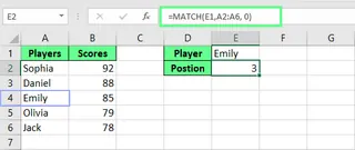Find the position of a text using the MATCH() function. Image by Author.

The AI-Powered Way: Simply ask Excelmatic: "What is Emily's position in the player list?" It’s as easy as asking a colleague.

Fuzzy Matching and Wildcard Matching in Excel

Sometimes, our data isn’t perfect. Typos, different spellings, or messy formats can make exact matches impossible. This is where fuzzy and wildcard matching come in, and where AI tools truly shine.

Fuzzy Match

Fuzzy matching finds records from different lists that are similar but not exactly the same. This is useful when dealing with typos like "Frank" vs. "Feank."

The Traditional Way (with Power Query): The standard Excel method for this is powerful but involves a multi-step process using Power Query.

Step 1: Convert data into tables

• Select your first list (e.g., Customer Orders), press Ctrl + T.
• Select your second list (e.g., Loyalty Program Members), press Ctrl + T.

Step 2: Load data into Power Query

• Select the first table, go to Data > Get Data > From Table/Range.
• Click Close & Load.
• Repeat for the second table.

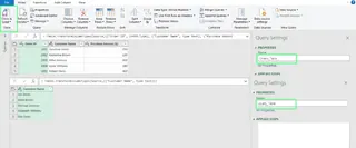Load the tables in Power Query. Image by Author.

Step 3: Merge tables using fuzzy matching

• Go to Data > Get Data > Combine Queries > Merge.
• Select your two tables and the columns to match.
• Check the Use Fuzzy Matching box and set a similarity threshold (e.g., 0.3).

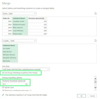Use fuzzy match to merge the tables. Image by Author.

Step 4: Expand the matched data

• Click the expand icon on the new column, select the fields you need, and click OK.
• Close & Load the results back into Excel.

Tables merged using the fuzzy match. Image by Author.

The AI-Powered Way: A Single Sentence The Power Query method is robust but complex. With Excelmatic, this entire process is simplified into one step.

• Upload your file with both lists.
• Ask: "Compare the 'Customer Orders' list with the 'Loyalty Program Members' list and find matching names, even if they have typos."

That's it. Excelmatic handles the complex logic of fuzzy matching behind the scenes, saving you time and effort.

Wildcard Match

Wildcard matching helps find values when you only know part of the text.

• * matches any number of characters (e.g., Jo* matches "John" and "Jonathan").
• ? matches just one character (e.g., J?ck matches "Jack" but not "Jake").

The Formula Way: To find the position of a person whose name ends with "e," you would use:

=MATCH("*e", A2:A11, 0)

The formula returns 3 because the name "Charlie" is the third entry and ends with "e."

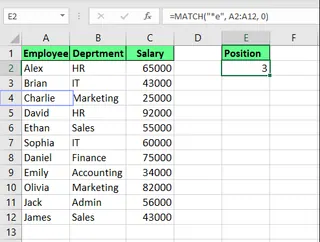Find the position using wildcards. Image by Author.

The AI-Powered Way: Instead of remembering wildcard syntax, just describe what you want. Ask Excelmatic: "Find the position of a name that ends with the letter e."

Combining MATCH() with Other Excel Functions

MATCH() truly shines when paired with other functions to create dynamic lookups. However, this is also where formulas can become long and difficult to debug.

Combining MATCH() with INDEX()

The INDEX() and MATCH() combination is a classic, flexible alternative to VLOOKUP(). It can look up values in any direction.

The Formula Way: To find Brian’s score from a list of players and scores, you would nest MATCH() inside INDEX():

=INDEX(B2:B11, MATCH("Brian", A2:A11, 0))

Here, MATCH() finds Brian's position (2), and INDEX() retrieves the value from the 2nd position in the score column (B2:B11).

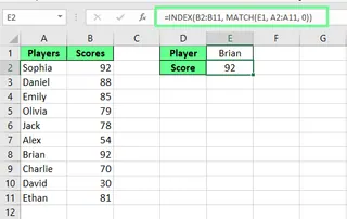Combine INDEX() and MATCH(). Image by Author.

The AI-Powered Way: Why build a two-part formula when you can just ask for the final answer? With Excelmatic, you'd ask: "What is Brian's score?" The AI handles the entire lookup process for you.

Using MATCH() for dynamic column selection in VLOOKUP()

A common limitation of VLOOKUP() is its static col_index_num. If you insert a column, the formula breaks. MATCH() can make it dynamic.

The Formula Way: To find Emily's "Team" name without hardcoding the column number, you can use:

=VLOOKUP(F1, A2:C12, MATCH("Team", A1:C1, 0), FALSE)

Here, MATCH("Team", A1:C1, 0) finds that "Team" is in the 3rd column, feeding that number into VLOOKUP().

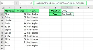Combine VLOOKUP() and MATCH(). Image by Author.

The AI-Powered Way: Again, focus on the goal, not the formula. Just ask Excelmatic: "What is Emily's team name?" The AI finds the right data regardless of column order.

Case-sensitive MATCH() using EXACT()

By default, MATCH() is not case-sensitive. To force a case-sensitive search, you need to combine it with the EXACT() function in an array formula.

The Formula Way: This is an advanced technique. The formula looks like this:

=MATCH(TRUE, EXACT(A2:A7, D2), 0)

Because this is an array formula, you must press Ctrl + Shift + Enter to make it work. It's powerful but easy to forget.

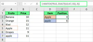Combine EXACT() and MATCH(). Image by Author.

The AI-Powered Way: Complex array formulas are a prime candidate for AI simplification. With Excelmatic, you simply add the condition to your request: "Find the position of 'Emily', making sure it is a case-sensitive match."

Final Thoughts

The MATCH() function, especially when combined with other functions, is a cornerstone of advanced Excel work. Mastering it can save you loads of time and make your spreadsheets more dynamic.

However, the landscape of data analysis is changing. AI agents like Excelmatic demonstrate that you no longer need to be a formula expert to get expert results. For complex tasks like fuzzy matching or dynamic lookups, a simple question in plain English can now replace a complicated, multi-step formula.

Learning the traditional methods is still valuable, but embracing Excelmatic can make you faster, more efficient, and free you up to focus on what the data actually means for your business decisions.

Ready to simplify your Excel data lookups? Try Excelmatic today and experience the power of AI-driven data analysis without complex formulas.

Excel FAQs

Can I compare two columns for matches and differences?

Traditional Way: Yes, you can use a combination of ISNA() and MATCH(). The formula =IF(ISNA(MATCH(B1,A1:A6,0)),"Not Present","Present") checks if a value from column B exists in column A.

AI-Powered Way: With Excelmatic, upload your file and ask, "Show me which values in column B are also present in column A."

How to handle errors when using MATCH()?

When the MATCH() function can’t find a value, it returns an #N/A error.

Traditional Way: To replace it with a custom message, wrap your formula in the IFERROR() function: =IFERROR(MATCH("Apple", A1:A5, 0), "Not Found")

AI-Powered Way: AI tools like Excelmatic are designed to give clean, human-readable answers. If a value isn't found, it will simply tell you "Not Found" or a similar clear message, eliminating the need for error-handling formulas.