Key Takeaways
- Excel error messages like #DIV/0! and #N/A make business reports look unprofessional and confuse stakeholders who need clear data insights
- Excelmatic's AI approach eliminates the need for complex IFERROR formulas - simply describe what errors to fix and what to replace them with
- The platform handles bulk error cleaning instantly, saving hours of manual formula writing and debugging for sales reports and financial dashboards
- For business users who need clean, presentable data without technical Excel skills, Excelmatic provides the fastest error-cleaning solution
Error messages like #DIV/0! or #N/A are a common and annoying sight in Excel. They make your reports look unprofessional and can be confusing for anyone trying to understand your data. Personally, I don’t like seeing these error messages in my workbooks, and I expect you feel the same way.
The good news is that there are powerful ways to manage them. In this guide, we'll explore two effective methods: the classic, formula-based approach using the IFERROR() function, and a modern, AI-powered alternative that can get the job done without writing a single formula.
Method 1: The Traditional Fix with the IFERROR() Function
For years, the go-to solution for handling errors has been the IFERROR() function. Let's break down how it works.
What Is the Excel IFERROR() Function?
The Excel IFERROR() function allows you to catch and handle errors in your formulas. Instead of displaying error messages like #DIV/0! or #N/A, IFERROR() lets you show a custom result or a more user-friendly message. This helps keep your spreadsheets looking clean and makes them easier to understand.
Excel IFERROR() Syntax
The IFERROR() function requires two arguments:
IFERROR(value, value_if_error)
value: The formula or expression you want to check for errors (e.g.,A1/B1).value_if_error: The value to return if an error is found (e.g., "Error" or 0).
How to Use Excel IFERROR() in Formulas
You can wrap almost any formula that might return an error inside IFERROR(). Here’s how you would apply it to a common division scenario:
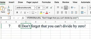
=IFERROR(A1/B1, "Don't forget that you can't divide by zero!")

If cell B1 contains a zero or is blank, Excel would normally display a #DIV/0! error. With IFERROR(), it will show your custom message instead, making your sheet much tidier.
Using Excel IFERROR() with Other Functions
IFERROR() is incredibly useful when combined with lookup functions like VLOOKUP, which often produce #N/A errors when a value isn't found.
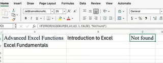
=IFERROR(VLOOKUP(A1:A3, B1, 1, FALSE), "Not found")

If VLOOKUP() cannot find a match, the formula will return "Not found" instead of the jarring #N/A error. This is a classic technique for building robust and user-friendly lookup tables.
Method 2: The AI-Powered Solution with Excelmatic
While IFERROR() is a powerful tool, what if you could achieve the same result without memorizing any functions? This is where AI Excel Agents like Excelmatic come in.

Excelmatic is an AI assistant that understands plain language. Instead of writing formulas, you simply upload your file and describe the task you want to perform.
Here’s how you would solve the same error-handling problems using Excelmatic:
- Upload your Excel file to the Excelmatic platform.
- State your request in plain language.
For the division-by-zero problem, your request would be as simple as:
In the results column, if there is a #DIV/0! error, replace it with 'Cannot divide by zero'.
For the VLOOKUP scenario, you would say:
For all #N/A errors in the 'Lookup Results' column, replace them with 'Not found'.
Excelmatic processes your command and instantly updates the entire column, handling all errors for you. There's no need to write, copy, or drag formulas.
Comparison: IFERROR() vs. Excelmatic
Both methods achieve the goal of cleaning up errors, but they cater to different workflows. Here’s a head-to-head comparison:
| Feature | IFERROR() Function (Manual) |
Excelmatic (AI-Powered) |
|---|---|---|
| How it Works | Manually wrap your existing formula inside IFERROR(). |
Describe your desired outcome in plain language. |
| Speed | Fast for single cells, but can be tedious for large datasets. | Instantaneous, even for thousands of rows. |
| Ease of Use | Requires knowledge of Excel syntax and function nesting. | As easy as sending a message. No formulas to remember. |
| Flexibility | Excellent for cell-by-cell control and dynamic calculations. | Ideal for batch processing, data cleaning, and analysis. |
| Learning Curve | Moderate. You need to understand how and when to use it. | Virtually none. If you can describe it, you can do it. |
When to Use Which Method
- Use
IFERROR()when you are building a dynamic template where values will change frequently and you need the error handling to be an integral part of the worksheet's logic. It's also a fundamental skill for any advanced Excel user. - Use Excelmatic when you have a dataset that needs quick and efficient cleaning. It's perfect for one-off tasks, handling large reports, or for business users who want to focus on the insights, not the technical implementation.
Conclusion
By mastering error-handling techniques, you can create cleaner, more professional, and user-friendly spreadsheets. The IFERROR() function is a powerful and essential tool in any Excel user's arsenal, giving you direct control over your formulas.
However, as technology evolves, so do our methods. Excelmatic offers a compelling alternative for business professionals, delivering the same high-quality results with unparalleled speed and simplicity. By leveraging plain language commands, you can now manage errors and perform complex data cleaning tasks in a fraction of the time.
The best approach depends on your specific needs, but for sales teams, marketing analysts, and operations managers who need clean data fast without technical hurdles, Excelmatic provides the most efficient path to professional-looking reports.
Ready to clean up your Excel errors without the formula complexity? Try Excelmatic today and experience the power of AI-driven data cleaning for your business reports.


