Key takeaways:
- The traditional
VLOOKUPfunction in Excel is powerful but rigid, error-prone, and requires manually counting columns, making data lookups tedious and fragile. - Excel AI tools like Excelmatic replace complex formulas with natural language. You can simply describe the data you want to find or merge, and the AI handles the entire lookup process automatically.
- Using Excelmatic for data lookups eliminates
#N/Aerrors, handles complex joins effortlessly, and allows for flexible, conversational analysis, turning a 30-minute task into a 30-second query.
Problem background & pain points
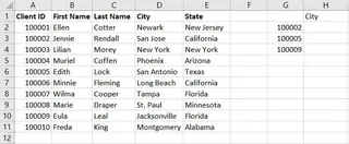
Imagine this common scenario: you have a master list of all your company's clients in an Excel sheet, complete with columns for Client ID, Name, City, and State. It's a huge table with thousands of rows.
Now, your manager hands you a small, separate list containing just a handful of Client IDs and asks you to "quickly pull the city for each of these clients."
If you're an Excel user, one function immediately comes to mind: VLOOKUP. It's the classic tool for this job—matching a value from one list to another and retrieving related data. But let's be honest, "quickly" is rarely part of the VLOOKUP experience.
First, you have to remember the exact syntax. Then, you need to make sure your lookup value is in the first column of your data range. You have to manually count which column number contains the "City" data. What if it's the 15th column? You count. What if someone adds a new column to the master list next week? Your formula breaks. And then there's the dreaded #N/A error that pops up for any ID that isn't found, making your report look messy and unprofessional.
This simple request to "pull some data" spirals into a frustrating exercise of writing, debugging, and protecting a fragile formula. For a task that feels like it should be simple, the manual process is surprisingly complex and full of potential pitfalls.
The Traditional Excel Solution: Steps and Limitations
For decades, VLOOKUP has been the go-to function for this task. It searches for a value vertically down the first column of a table and returns a corresponding value from a specified column in the same row.
The syntax looks like this:
=VLOOKUP(lookup_value, table_array, col_index_num, [range_lookup])
Let's break down how you'd solve the client city lookup problem manually.
Step 1: Identify the lookup_value
This is the value you want to find. In our example, it's the first Client ID in your small list, say in cell G2.
Step 2: Define the table_array
This is the entire range of your master client data, for example, A1:E11. You must ensure the Client ID is the first column in this range. You'll also want to lock this range with dollar signs ($A$1:$E$11) so it doesn't shift when you drag the formula down.
Step 3: Determine the col_index_num
Now, you manually count the columns in your table_array to find the one containing the city. If 'Client ID' is column 1, 'First Name' is 2, 'Last Name' is 3, then 'City' is column 4. You enter 4 into the formula.
Step 4: Set the range_lookup
You almost always want an exact match, so you enter FALSE. This tells Excel to only return a result if it finds the exact Client ID.
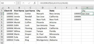
The final formula in cell H2 would be:
=VLOOKUP(G2, $A$1:$E$11, 4, FALSE)
You then drag this formula down for all the other Client IDs in your list.
The Limitations of the VLOOKUP Method
While it gets the job done, this traditional approach is plagued with issues:
- It Only Looks Right:
VLOOKUPcan only search for a value in the leftmost column of your table array. If you need to look up a Client ID and find a value in a column to its left,VLOOKUPis useless. You'd have to rearrange your data or switch to a more complexINDEX(MATCH)combination. - Fragile Column Index: The
col_index_numis a hardcoded number. If you or a colleague inserts a new column in the master data (e.g., a "Join Date" column between 'Last Name' and 'City'), your column count of4is now wrong. It will start pulling the wrong data (or an error) without warning, silently corrupting your report. - Ugly Errors: If a Client ID from your list doesn't exist in the master table,
VLOOKUPreturns an#N/Aerror. To create a clean report, you have to wrap your formula in another function, likeIFERROR, making it even longer and more complex:=IFERROR(VLOOKUP(...), "Not Found"). - Returns Only the First Match: If your data has duplicate Client IDs,
VLOOKUPwill find the first one in the list and stop. It has no built-in way to show you all possible matches, which can be misleading. - Not Intuitive: For anyone who doesn't "live" in Excel, the syntax is not self-explanatory. Explaining
col_index_numor whyFALSEis important to a new team member is a common training headache.
The New Approach: Using Excel AI (with Excelmatic)
Instead of memorizing formulas and manually structuring your data, what if you could just tell Excel what you want to do? This is exactly what Excel AI agents like Excelmatic are designed for. You upload your file and use plain language to perform complex tasks like data lookups.

Here’s how you can solve the exact same problem in a fraction of the time.
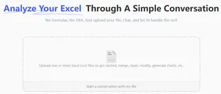
Step 1: Upload Your Data File
First, you simply upload your Excel workbook containing both the master client list and the short list of IDs you need to look up. Excelmatic accepts Excel (.xlsx, .xls) and CSV files. For best results, ensure your data has clear column headers like "Client ID," "City," etc.
Step 2: Describe Your Goal in Plain Language
Instead of writing a formula, you type a request in the chat interface. You can be direct and specific about what you want to achieve.
Here are a few examples of prompts you could use:
- "I have two sheets, 'Client Master' and 'Lookup List'. For each 'Client ID' in 'Lookup List', find the corresponding 'City' from the 'Client Master' sheet and add it as a new column."
- "Merge my two tables based on the common 'Client ID' column."
- "Using the client ID, pull the city and state for the clients in the second sheet."
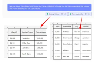
Excelmatic's AI understands the relationship between your tables and the intent behind your request.
Step 3: Review and Iterate on the Results
In seconds, Excelmatic will present you with the result—a new table showing your original lookup list with the "City" column correctly populated. There are no formulas to check or errors to fix.
The best part is that this is a conversation. You can easily refine or expand your request. For instance, you could follow up with:
- "Great. Now also add the 'State' column."
- "Filter this list to only show clients from 'New York'."
- "Can you sort the final list alphabetically by city?"
This conversational approach to data analysis is impossible with static formulas. It allows you to explore your data and answer follow-up questions on the fly.
Step 4: Export Your Clean Data
Once you're happy with the result, you can download the newly created table as a clean Excel file with one click. The data is ready to be shared or used in a presentation, with no messy formulas or #N/A errors.
Dialogue Example
Here’s what a typical interaction with Excelmatic might look like for this task:
User: I've uploaded a file with two tabs: 'All Clients' and 'IDs to Check'. I need to find the city for each client listed in 'IDs to Check' by matching their 'Client ID' with the data in the 'All Clients' tab.
Excelmatic: Understood. I have merged the data for you. I've added the 'First Name', 'Last Name', 'City', and 'State' columns to your 'IDs to Check' list based on the 'Client ID'. Would you like me to remove any of these new columns?
User: This is perfect, but I only need the 'City' column for now. Please remove the others.
Excelmatic: Done. The table now shows only the 'Client ID' and its corresponding 'City'. You can download the updated Excel file below.
VLOOKUP vs. Excelmatic: A Quick Comparison
| Feature | Traditional VLOOKUP |
Excelmatic (Excel AI) |
|---|---|---|
| Time to Complete | 5-15 minutes (writing, debugging, cleanup) | < 1 minute |
| Learning Curve | Moderate; requires understanding syntax, absolute references, and error handling. | Minimal; requires ability to describe a business need in plain language. |
| Flexibility | Low. Breaks if columns are inserted/deleted. Only looks right. | High. Understands context. Can look left, right, and merge complex data. |
| Error Handling | Manual. Requires IFERROR to manage #N/A errors. |
Automatic. Returns clean data, clearly indicating which values were not found. |
| Follow-up Questions | Requires writing entirely new formulas or manually filtering. | Simple. Just ask a follow-up question in the chat. |
FAQ
1. Do I need to know any Excel formulas to use Excelmatic?
No. That's the main advantage. You don't need to know VLOOKUP, INDEX(MATCH), or any other formula. You just need to be able to describe the outcome you want in plain language.
2. Is my data safe when I upload it to Excelmatic? Data privacy and security are top priorities. Excelmatic uses secure connections and infrastructure to process your files. For specific details on data handling and privacy, it's always best to consult the official privacy policy on the website. Your original file is not modified.
3. What if my lookup column isn't the first column in my data?
This is a classic VLOOKUP limitation that Excelmatic completely eliminates. Because you're using natural language, the AI understands which columns to match regardless of their position in the table. You can just say "Match 'Client ID' from Sheet1 with 'Customer Number' in Sheet2."
4. Can Excelmatic handle approximate matches, like VLOOKUP's TRUE option? Yes. You can ask it to find the closest match. For example, you could ask, "For each sale amount, find the corresponding commission tier from the rate table, rounding down to the nearest tier."
5. What happens if a value I'm looking for doesn't exist?
Instead of returning an #N/A error, Excelmatic will simply leave the corresponding cell blank or you can instruct it on how to handle missing values, for instance by writing "Not Found". This results in a much cleaner and more professional-looking output from the start.
6. Can I use the formulas generated by Excelmatic in my own sheets? Yes. In addition to providing the final data, Excelmatic can also generate the exact Excel formula needed to perform the task. You can copy this formula and paste it into your own workbook, which is a great way to learn or to automate tasks within your existing files.
Take Action: Upgrade Your Excel Workflow with Excelmatic
Stop wasting time wrestling with fragile VLOOKUP formulas. The minutes you spend counting columns, locking cell references, and cleaning up #N/A errors add up to hours of lost productivity every month.
By embracing an Excel AI agent, you shift your focus from how to perform a task in Excel to what business question you want to answer. Looking up data becomes as simple as asking a question, giving you back valuable time to focus on more strategic analysis.
Ready to see for yourself? Try Excelmatic today. Upload one of the files you're currently working on and use one of the prompts from this article. Experience firsthand how a simple conversation can replace a complex formula.


