Key Takeaways
- Manual amortization schedules require complex financial formulas like PMT, IPMT, and PPMT that are time-consuming and prone to errors
- Traditional Excel methods demand technical expertise in cell references and formula dragging that distracts from financial analysis
- Excelmatic generates complete amortization tables instantly using simple English commands—no formulas needed
- For business professionals, AI automation provides faster, more reliable results than manual financial modeling
An amortization schedule provides a clear financial roadmap, showing how each loan payment splits between interest and principal until your debt is fully paid off. While it sounds complex, creating one in Excel is a powerful way to visualize your loan's lifecycle, make informed financial decisions, and even explore options for early payoff.
Traditionally, this meant building a complex table from scratch with financial formulas. But what if you could get the same result in seconds, just by asking?
In this article, you'll learn two effective methods for building a comprehensive amortization schedule in Excel. We'll first walk through the classic, manual approach using essential functions like PMT(), IPMT(), and PPMT(). Then, we'll introduce a modern, AI-powered solution using Excelmatic that delivers the same results instantly, without a single formula.
What Exactly Is an Amortization Schedule?
An amortization schedule is a complete table of periodic loan payments, showing the amount of principal and interest that comprise each payment until the loan is paid off at the end of its term.
When you take out a loan, several key elements determine how your payments work:
- Principal: The original amount borrowed that you must repay
- Interest: The cost of borrowing the money, calculated as a percentage of the principal
- Payment period: How often you make payments (monthly, bi-weekly, etc.)
- Loan term: The total time period over which you'll repay the loan
For most standard loans—like mortgages, auto loans, and personal loans—payments remain consistent throughout the term. However, what changes with each payment is the proportion that goes toward interest versus principal. In the early stages, a larger percentage of each payment covers interest. As you progress through the loan term, more of each payment reduces the principal balance.
The primary purpose of creating an amortization schedule is to provide transparency into your loan. It lets you see exactly how much interest you'll pay over time, how quickly you're building equity, and how additional payments might affect your loan timeline.
Method 1: The Traditional Way - Building a Schedule Manually
For those who want to understand the mechanics behind loan amortization, building a schedule manually in Excel is an excellent exercise. This method gives you full control but requires careful attention to formulas and cell references.
The Excel Functions and Formulas You Need to Know
Excel does not have a single built-in "amortization" function. Instead, you'll use a combination of financial functions:
PMT() function
The PMT() function calculates the total payment for a loan based on constant payments and a constant interest rate.
=PMT(rate, nper, pv, [fv], [type])
IPMT() function
The IPMT() function calculates the interest portion of a specific payment.
=IPMT(rate, per, nper, pv, [fv], [type])
PPMT() function
The PPMT() function calculates the principal portion of a specific payment.
=PPMT(rate, per, nper, pv, [fv], [type])
You will also need custom formulas for Remaining Balance, Cumulative Principal, and Cumulative Interest, and to be mindful of absolute ($A$1) vs. relative (A1) references to ensure your formulas work when copied down.
Step-by-Step Guide to Creating the Schedule Manually
Let's build an amortization schedule from scratch for a $250,000 loan over 30 years at 4.5% interest.
1. Entering loan data
Enter your loan details in dedicated input cells.
- Loan amount: $250,000 (cell B1)
- Annual interest rate: 4.5% (cell B2)
- Loan term: 30 years (cell B3)
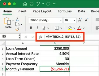 Setting up the loan input parameters. Image by Author.
2. Calculating the monthly payment
In cell B5, calculate the monthly payment using the PMT function: =PMT(B2/12, B3*12, B1). This will return -$1,266.71. The negative sign indicates a cash outflow.
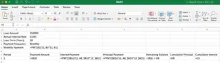 Setting up the column headers and formulas. Image by Author.
3. Creating the first row of the schedule
Set up your headers (Period, Payment, Interest, etc.) and enter the formulas for the first payment period. Remember to use absolute references ($B$1) for fixed inputs.
- Interest Payment:
=IPMT($B$2/12, A8, $B$3*12, $B$1) - Principal Payment:
=PPMT($B$2/12, A8, $B$3*12, $B$1) - Remaining Balance:
=$B$1+D8
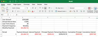 Showing the breakdown of the first payment. Image by Author.
4. Completing the schedule
Create the formulas for the second row, making sure to reference the previous row's values for cumulative and remaining balance calculations.
- Remaining Balance:
=E8+D9(Previous Balance + Current Principal) - Cumulative Principal:
=F8+D9(Previous Cumulative + Current Principal) - Cumulative Interest:
=G8+C9(Previous Cumulative + Current Interest)
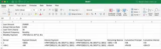 Setting up formulas that can be copied down. Image by Author.
Once the second row is set up correctly, select the entire row and drag the fill handle down 360 rows to complete the schedule.
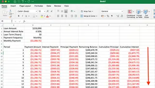 As you progress through the loan term, more of each payment goes toward principal rather than interest. Image by Author.
5. Verifying the final payment
If all formulas are set up correctly, the remaining balance after the final payment should be $0.00. Carefully check the final result to ensure accurate calculations.
As you can see, the manual method works perfectly, but it's a multi-step process that can be tedious and prone to errors if a reference is misplaced.
Method 2: The Smart Way - Using an AI Agent like Excelmatic

What if you could skip all the formulas and manual steps? With an AI Excel Agent like Excelmatic, you can. Excelmatic generates instant answers, charts, and insights for your data just by asking in plain language.
Instead of building the schedule cell by cell, you simply state your request.
Here’s how you would create the exact same amortization schedule with Excelmatic:
- Upload your file containing the loan parameters (or simply state them in your request).

- Ask your question in plain language.

- Get instant, accurate results without writing any formulas.

Excelmatic handles everything else. It instantly generates the complete, fully-formatted 360-payment schedule, with all columns calculated perfectly. There are no formulas to remember, no cell references to lock, and no risk of drag-and-fill errors.
When You Need Absolute References (And How Excelmatic Handles It)
In the manual method, you must use absolute references like $B$1 to lock the loan amount, interest rate, and term. Forgetting these dollar signs breaks the entire schedule when dragging formulas.
Traditional Approach Requires Technical Knowledge:
=IPMT($B$2/12, A8, $B$3*12, $B$1)-must remember all the $ symbols- High risk of error if references are incorrect
Excelmatic Approach:
Create an amortization schedule using the loan amount in B1, interest rate in B2, and term in B3
The AI automatically handles all reference locking without requiring you to master absolute reference syntax.
Comparing the Two Methods: Manual vs. AI
| Feature | Manual Excel Method | Excelmatic (AI Agent) Method |
|---|---|---|
| Speed & Efficiency | Slow; requires setup, formula entry, and dragging. | Instant; generates the full table in seconds. |
| Complexity | High; requires knowledge of PMT, IPMT, PPMT, and references. |
Low; uses simple, plain language commands. |
| Accuracy | Prone to human error (e.g., wrong cell reference, typos). | Highly accurate; eliminates formula and calculation errors. |
| Flexibility | Good, but changes require manual formula adjustments. | Excellent; easily handles follow-up questions for changes. |
Additional Things You Might Want to Consider
A standard schedule is just the beginning. To make your model more flexible, consider these scenarios:
Managing payment variations
Want to see how extra payments affect your loan?
- Manual Method: You'd need to add a new "Extra Payment" input cell and modify your principal and remaining balance formulas to account for it.
- Excelmatic Method: Simply ask a follow-up question: "Now show what happens if I make an extra $100 payment each month." The schedule will update instantly.
Enhancing readability and analysis
Proper formatting is key. You can use conditional formatting to highlight milestones, like when you’ve paid off half the principal. Both a manually created sheet and an Excelmatic-generated one can be formatted, but Excelmatic often applies logical formatting automatically.
Customizing for specific loan types
Different loans (e.g., mortgages with escrow, loans with balloon payments) may require adjustments. While you can add more columns and logic manually, an AI agent can often incorporate these complexities with a more detailed initial request.
Conclusion
Creating an amortization schedule in Excel gives you valuable insight into your loans. The manual method is a fantastic way to learn the financial mechanics behind your debt, and the skills you gain are widely applicable.
However, for speed, accuracy, and efficiency, modern AI tools like Excelmatic are a game-changer. They allow you to move from question to answer in seconds, freeing you to focus on analysis and decision-making rather than on the tedious process of building formulas.
Why spend hours building complex financial models when you can describe your needs in plain English and get perfect results instantly?
Try Excelmatic today and experience the future of financial modeling.
What is the difference between the PMT(), IPMT(), and PPMT() functions in Excel?
PMT() calculates the total periodic payment for a loan, while IPMT() gives only the interest portion of a specific payment, and PPMT() gives only the principal portion of a specific payment.
Why does my PMT() function return a negative number?
Excel uses a cash flow convention where money you pay out (like loan payments) shows as negative values, while money you receive shows as positive values.
Can I create an amortization schedule for bi-weekly payments instead of monthly?
Yes. In the manual method, adjust your rate calculation to annual rate/26 and the number of periods to years*26. With Excelmatic, you would simply specify "bi-weekly payments" in your request.
Can I create an amortization schedule for a loan with a variable interest rate?
Yes. Manually, you can create different sections in your schedule with updated interest rate values. With Excelmatic, you can specify the rate changes in your prompt (e.g., "rate is 5% for the first 5 years, then 6%").


